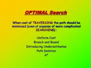
OPTIMAL Search
This document delves into the Uniform Cost Algorithm (UCA) and its integration with the Branch and Bound technique, emphasizing underestimation in heuristic searches. It presents how the UCA minimizes traversal costs and addresses limitations in finding optimal paths. By utilizing concepts like accumulated costs and heuristic estimates, the paper explores iterative methods to enhance search efficiency. Key principles include the importance of path deletion and the consequences of cost estimates on the search outcome, ultimately aiming for optimal solutions in complex search spaces.

OPTIMAL Search
E N D
Presentation Transcript
OPTIMAL Search Uniform Cost Branch and Bound Introducing Underestimates Path Deletion A* When cost of TRAVERSING the path should be minimized (even at expense of more complicatedSEARCHING) :
4 4 3 5 5 4 3 2 4 4 3 S 4 A D 2 5 5 A B C B D A E 4 5 S 5 2 4 4 G C E E B B F 2 4 5 4 4 5 4 4 D E F 3 D F B F C E A C G 3 4 3 4 G C G F 3 G Re-introduce the costs of arcs in the NET
S 3 4 4 3 A D 5 4 5 2 6 9 B 7 A 8 D E 5 4 5 4 5 4 11 10 11 12 13 C B 13 B F E E 3 B 13 F F C A C D E G C F G G G Uniform cost algorithm= uniformed best-first • At each step, select the node with the lowest accumul-ated cost.
(BY ACCUMULATED COST) Uniform cost algorithm: 1. QUEUE <-- path only containing the root; 2. WHILEQUEUE is not empty AND goal is not reached DO remove the first path from the QUEUE; create new paths (to all children); reject the new paths with loops; add the new paths and sort the entire QUEUE; 3. IF goal reached THEN success; ELSE failure;
S 1 1 5 5 A C 1 2 5 B 10 D 5 15 E 100 5 F 20 G 5 Problem: NOT always optimal! • Uniform cost returns the path with cost 102, while there is a path with cost 25.
S 2 3 A B 0.5 3.5 3 2 D 3 5 C 5 G 6 X ignore E G X ignore First goal reached The Branch-and-Bound principle • Use any (complete) search method to find a path. • Remove all partial paths that have an accumulated cost larger or equal than the found path. • Continue search for the next path. • Iterate.
S 1 1 5 5 A C 1 2 5 B 10 D 5 15 E 100 5 F 20 G 5 102 25 A weak integration of branch and bound in uniform cost: • Change the termination condition: • only terminate when a path to a goal node HAS BECOME THE BEST PATH.
Optimal Uniform cost version: 1. QUEUE <-- path only containing the root; 2. WHILE QUEUE is not empty ANDfirst path does not reach goal remove the first path from the QUEUE; create new paths (to all children); reject the new paths with loops; add the new paths and sort the entire QUEUE; 3. IF goal reached THEN success; ELSE failure; (by accumulated cost)
S 3 4 A D S 4 A A D 7 8 B D S A D D 7 8 9 6 A B D E S A D 9 7 8 A E E B D 10 11 B F Example:
S A D 9 8 A D B B E 11 10 B F 11 12 C E S A D 9 A D D B E 11 10 B F 11 12 10 C E E S A D A A D B E 11 10 B F 11 13 12 10 C E E B S A D A D B E 11 10 B F 11 13 12 C E E E B 15 14 B F
S A D A D B E 11 B F F 11 13 12 C E E B 15 14 13 B F G S A D A D B E B B F 11 13 12 C E E B 15 14 15 15 13 B F A C G S A D A D B E B F 13 C E E E B 14 15 15 15 13 16 B F 14 D F A C G Don’t stop yet! STOP!
Properties of extended uniform cost : • Optimal path: • If there exists a number > 0, such that every arc has cost , and if the branching factor is finite, • Thenextended uniform cost finds the optimal path (if one exists). • Memory and speed: • In the worst case, at least as bad as for breadth-first: • needs additional sorting step after each path- expansion ! • How to improve ?
f(path) = cost(path) + h(endpoint_path) + Extension with heuristic estimates: • Replace the ‘accumulated cost’ in the ‘extended uniform cost’ algorithm by a function: • where: cost(path) = the accumulated cost of the partial path h(T) =a heuristic estimate of the cost remaining from T to a goal node f(path) =an estimate of the cost of a path extending the current path to reach a goal.
G 3 C F 4 4 B 5 E 4 2 10.4 6.7 A B C 4 5 D A 11 S 4 G 8.9 3 F 6.9 S 3 D E Example: Reconsider the straight-line distance: • h(T) = the straight-line distance from T to G
S 3 + 10.4 = 13.4 4 + 8.9 = 12.9 A D S 13.4 A D D 9 + 10.4 = 19.4 6 + 6.9 = 12.9 A E S 13.4 A D 19.4 A E E 11 + 6.7 = 17.7 B 10 + 3.0 = 13.0 F S 13.4 A D 19.4 A E 17.7 B F F 13 + 0.0 = 13.0 G STOP!
(by f = cost + h) Estimate-extended Uniform cost algorithm: 1. QUEUE <-- path only containing the root; 2. WHILE QUEUE is not empty ANDfirst path does not reach goal remove the first path from the QUEUE; create new paths (to all children); reject the new paths with loops; add the new paths and sort the entire QUEUE; 3. IF goal reached THEN success; ELSE failure;
IF for all T: h(T) is an UNDERestimate of the remaining cost to a goal node • THEN estimate-extended uniform cost is optimal. S includes underestimated remaining cost 13.4 A D 19.4 A E 17.7 B F with real remaining cost, this path must at least be 13.4 13 G G Optimality • With the same condition on the arcs-costs and on the branching factor: • Intuition:
2 3 1 1 3 2 1 1 Real remaining costs A B C 1 1 Over- estimate 1 5 2 4 1 1 1 S D E G 3 2 1 1 3 1 4 2 1 1 F H I 1+3 2+2 3+1 A A B B C C 1+5 4 S D G 1+4 Not the optimal path! F More on underestimates: • Example: • If h is NOT an underestimate:
2 3 0 1 1 0 1 1 Real remaining costs A B C 1 1 Under- estimate 1 2 2 1 1 1 1 S D E G 3 2 1 1 2 1 3 1 1 1 F H I 1+1 2+0 3+0 A A B B C C 1+2 4 3 ! E E G S D D G 1+3 F More on underestimates: • Example: • If h is an underestimate: 2+1 Bad underestimates always get cor- rected by increasing accumulated cost
Speed and memory • In the worst case: no improvement over ‘branch and bounded extended uniform cost’ • Just take h = 0 everywhere. • For good heuristic functions: search may expand much less nodes ! • See our running example. • BUT: the cost of computing such functions may be high • Trade-off
S 3 4 A A D 7 8 B D Accumulated distance • Principle: • the minimum distance from S to Gvia I = (min. dist. from S to I) + (min. dist. from I to G) An orthogonal extension:path deletion • Discard redundant paths: • in the ‘branch and bound extended uniform cost’ : X discard !
S A D Q P 7 8 9 6 A B D E More precisely: • IF the QUEUE contains: • a path P terminating in I, with cost cost_P • a path Q containing I, with cost cost_Q • cost_Pcost_Q • THEN • delete P X
S 3 4 A D S 4 A D 7 8 B D X S A D 7 9 6 A B D E X X S A D 7 A E B D X X 10 11 B F X
S A D A D B E X X 10 B F 11 12 C E X X S A D A D B E X X B F 11 C E X 13 X G Note how this optimization reduces the number of expansions VERY much, compared to ‘branch and bound extended uniform cost’. 5 expansions less !
A* search • IS: • Branch and bound extended, • Heuristic Underestimate extended, • Redundant path deletion extended, • Uniform Cost Search. • Note that redundant path deletion is based on the accumulated costs only, so that there is no problem combining it with heuristic underestimates.
A* algorithm: 1. QUEUE <-- path only containing the root; 2. WHILE QUEUE is not empty ANDfirst path does not reach goal remove the first path from the QUEUE; create new paths (to all children); reject the new paths with loops; add the new paths and sort the entire QUEUE; IFQUEUE contains path P terminating in I, with cost cost_P, and path Q containing I, with cost cost_Q AND cost_Pcost_Q THEN delete P 3. IF goal reached THEN success; ELSE failure; (by f = cost + h)
S 3 + 10.4 = 13.4 4 + 8.9 = 12.9 A D S 13.4 A D 9 + 10.4 = 19.4 6 + 6.9 = 12.9 A E X Only difference is here. S 13.4 A D A E X B 10 + 3.0 = 13.0 F 11 + 6.7 = 17.7 S 13.4 A D A E STOP! X 17.7 B F 13 + 0.0 = 13.0 G