Progress toward a viable HIM-based coupled model
240 likes | 257 Vues
This article discusses the progress made in developing a viable HIM-based climate model, including code conversion, coupling of ocean and sea ice models, handling of pressure gradients and mixed layer dynamics, and addressing parameter tuning conflicts. It also compares the HIM-based model with MOM-based models and highlights the need for further tuning to reduce biases and improve simulation results.

Progress toward a viable HIM-based coupled model
E N D
Presentation Transcript
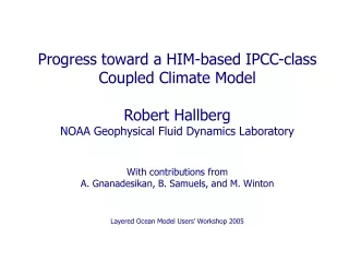
Progress toward a HIM-based IPCC-classCoupled Climate ModelRobert HallbergNOAA Geophysical Fluid Dynamics LaboratoryWith contributions from A. Gnanadesikan, B. Samuels, and M. WintonLayered Ocean Model Users’ Workshop 2005
Progress toward a viable HIM-based coupled model • Code conversion to F90/FMS • Coupling C-grid ocean to B-grid Sea ice model • Full nonlinear equation of state used everywhere except as the vertical coordinate • Pressure gradients • Mixed layer dynamics • Shear Richardson Numbers • Parameter tuning conflicts & challenges • Shear Richardson number – EUC and Overflows • Excessive Buffer Layer Mixing • Comparisons between HIM & MOM-based coupled model solutions.
HIM Code conversion to F90/FMS • F90-HIM code exactly reproduces C-HIM code answers. • F90 code uses either static or dynamic memory allocation. • Model with static allocation twice as fast as with dynamic on O3k • Uses macros so this does not require prevasive code duplication • C code is a few percent faster than static F90 code on 1 CPU. • Probably from reuse of limited scope temporary variables. • F90/FMS code scales slightly better than C code. • Less synchronization (8-way messages vs. 2x2-way messages) • Buffered, multithreaded I/O • C code has a much smaller memory footprint than FMS/F90 code. • Identical interface to MOM4 • HIM interface accommodates multiple staggerings of wind stresses. • Same run-time specification of diagnostics as MOM4.
Gnanadesikan et al., subm. J. Climate The GFDL Sea Ice Model (SIS) • State-of-the-art dynamical/thermodynamical sea-ice model • 5 ice thickness categories + leads • 3 vertical levels • Elastic-viscous-plastic ice internal forces (rheology) • B-Grid Sea Ice / C-Grid Ocean Coupling Issues: • Stress • Ice-ocean stress calculated on a B-grid, then averaged to a C-grid • Open-ocean stress goes directly from A-grid to C-grid • No ice flow through narrow channels • May also occur because of proper ice dynamics MOM4/SIS Sea Ice Mass
Using Fully Nonlinear Equation of State • Vertical coordinate – 45 s2000 layers plus a bulk mixed layer and buffer layer • Horizontal mixing is still along coordinate surfaces. • Pressure Gradients: • In-situ density with thermobaric compensation described by Hallberg, Ocean Modelling, 2005 & LOM Workshop 2004 • Mixed Layer Dynamics • Integral Potential Energy Budgets based on local fits of and • Shear Richardson Numbers • Based on in-situ values of and
Annual Maximum Mixed Layer Depth Convective adjustment based on s0 Convective adjustment based on s0or s2000 Log of maximum mixed layer depth in m
Annual Mean Coupled Model SST Anomalies Model still requires substantial tuning to reduce biases.
Seasonal Cycle of Coupled Model SST Errors JFM AMJ JAS OND
Mixed Layer Buffer Layer Excessive Mixing between Buffer and Mixed Layers Late Winter Buoyancy Profile 6 AM Profile 1 PM Profile 6 AM Profile • The combination of seasonal and higher frequency (diurnal or storm/calm cycle) leads to excessive mixing in the buffer layer. • Adding resolution to the sub-mixed-layer region should help substantially. • Not an issue if the resolution does not track the mixed layer base (e.g. in HYCOM). Seasonal Restratification Mixed Layer
Shear Richardson Number Mixing and the Equatorial Under Current Without parameterized mixing, the EUC is much stronger and shallower. June, Year 6 June, Year 6
Impact of Richardson Number Dependent Mixing on the Equatorial Undercurrent at 140°W June, Year 6 June, Year 6
Comparison between HIM- and MOM-based Coupled Models Topography for HIM and MOM based 1° coupled models. MOM HIM
CM2.0/HIM & CM2.0/MOM Annual Mean SST Errors CM2.0/HIM (untuned) CM2.0/MOM4 (tuned) • Similar error patterns – errors possibly due to atmospheric forcing. • Differences in errors – oceanographic impact on the climate simulation. • Coupled models with 2 different atmospheres confirms this • CM2.0: B-grid dynamical core atmosphere • CM2.1: S.J. Lin’s finite volume dynamical core atmosphere (FVCore)
SST Error in 3RD Pentad MOM HIM CM2.0 CM2.0 CM2.1 CM2.1
Surface Air Temperature Differences in two pairs of coupled models CM2.0 (B-grid atmos) CM2.1 (FVCore atmos) HIM SAT-MOM SAT in 3rd Pentad
ENSO in MOM and HIM Based Coupled Models CM2.1MOM SST on Equator CM2.1HIM SST on Equator
Summary • GFDL has complementary 1° HIM- and MOM- based coupled climate models. • Multiple models help identify source of biases. • Should provide invaluable estimates of the robustness of results. • Significant recent HIM developments to achieve a coupled model: • Conversion of code to FMS/F90. • Nonlinear equation of state used everywhere in physical equations. • Multiple fully coupled models assembled and run for decades. • Much work remains to tune HIM-based coupled model. • Multiple buffer layers to avoid excessive mixing. • Reconciliation of conflicts between overflow and EUC entrainment parameterizations. • Mixed layer and eddy parameter tuning.
Sea Ice Concentration Error 3RD Pentad MOM HIM CM2.0 CM2.0 CM2.1 CM2.1
Year 17; 2 km Depth Salinity and Velocity Levitus Salinity CM2.0MOM CM2.0HIM