Download
1 / 14
460 likes | 1.48k Vues
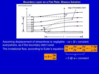
Boundary Layer on a Flat Plate: Blasius Solution. from Kundu’s book. Assuming displacement of streamlines is negligible → u = U = constant everywhere, as if the boundary didn’t exist. H. z. The irrotational flow, according to Euler’s equation:. = 0 @ u = constant.

E N D
Boundary Layer on a Flat Plate: Blasius Solution from Kundu’s book Assuming displacement of streamlines is negligible →u = U = constant everywhere, as if the boundary didn’t exist H z The irrotational flow, according to Euler’s equation: = 0 @ u = constant
The complete set of equations for Boundary Layer are: from Kundu’s book H z
The velocity profile in the boundary layer can be obtained with a SIMILARITY SOLUTION – following Blasius, a student of Prandtl Velocity distributions at various x can collapse into a single curve if the solution has the form For similarity solution, use streamfunction: from Kundu’s book Using similarity form above: H z Using the definition:
f and its derivatives do not explicitly depend on x : initial and boundary conditions: Can be valid only if: Blasius equation
% uses Matlab ODE45 - Runge-Kutta method ti = 0.0; % start of integration tf = 7.0; % final value of integration bcinit = [0.0 0.0 0.33206]; % initial values [eta f] = ode45('state',[titf],bcinit); ================== function stst = state(eta,f) stst = [ f(2) , f(3) , -0.5*f(1)*f(3)]';
Boundary Layer Thickness Distance η where u = 0.99 U η = 4.9 Rex
displacement thickness momentum thickness
Skin Friction Local wall shear stress using: @z = 0
Skin Friction Local wall shear stress Wall shear stress then changes as x -½, i.e., decreases with increasingx
Local shear stress at wall can be expressed in terms of the local drag coefficient and the drag force per unit width of plate of length L So the drag force is proportional to the 3/2 power of velocity (U 2/U 1/2) For high Re the drag force is proportional to the square of velocity Now, the overall drag coefficient is defined as: overall drag coefficient is average of local drag coefficient
http://www.symscape.com/node/447 Breakdown of Blasius solution Transition from laminar to turbulent region occurs at Recr(~106) Transition depends on a) surface roughness and b) shape of leading edge Boundary layer grows faster in the turbulent region because of macroscopic eddies