One Variable Input
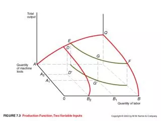
One Variable Input. First we will look at the production process when one input can vary (change its level) and all other inputs are held at a constant level (e.g. fixed). Production Function One in Tabular Form. Max Tpp. How else can we represent a Production Function?.

One Variable Input
E N D
Presentation Transcript
One Variable Input First we will look at the production process when one input can vary (change its level) and all other inputs are held at a constant level (e.g. fixed).
How else can we represent a Production Function? Mathematical Notation: Y = f(X) Example: Y = 10X + 6X2 - X3 X is input. Y is output.
Terms to Know • Total Physical Product TPP or Y • Average Physical Product APP or Y/X • Marginal Physical Product MPP or Y/ X
X Represents INPUT Level Y Represents Output Level Means “Change In”
Average Physical Product (APP) APP is a measure of the average amount of output produced per unit of variable input supplied. We must consider APP to address the question of whether it is worthwhile to produce anything at all. Why?
Deciding to Produce If the average amount of product produced per unit of input used is worth less (in money) than it costs us to buy a unit of input, we shouldn’t produce.
Should we produce where APP is at a maximum? Generally we don’t produce where APP is at a max. We’ll discuss why when we look at MPP. For now, though, it is important to remember that we do need to look at APP to decide if it is a good idea to produce at all.
Marginal Physical Product (MPP) MPP is the change in output associated with using one more unit of input. It tells you how much extra product you get if you use one extra input. MPP is important for finding the amount of input that should be used to maximize profits.
The Geometry of Production APP is the slope of the line going from the origin (0,0) to the production function. MPP is the slope of the tangent line to the function. We approximate it for discrete changes with the secant line (e.g. line connecting two points on the function).
APP and the Geometry of Production output text slope is rise over run Y X input
MPP and the Geometry of Production output text input Tangent lines
APP = MPP when APP is at its maximum output text input
MPP as a secant output text Y X input
Where is the maximum MPP? output text max MPP at inflection point input
Law of Diminishing Returns As the number of units of the variable input increases, other inputs held constant, after a point the MPP of the variable input starts to decline. Note: This law refers to marginal physical product. Eventually, MPP will fall.
A Function . . . . . . may exhibit increasing returns for a while (MPP rising) or constant returns (MPP steady) for a while, but eventually MPP must fall. If MPP didn’t eventually fall, there would be an incentive to produce an infinite amount of output.
Repeat The Law of Diminishing Returns refers to marginal physical product, not total physical product.
Where do diminishing returns begin? output text at max MPP input
Three Stages of Production We divide the production function into three stages of production.
Stage I • APP is increasing • MPP > APP • TPP is increasing
Stage II • APP is decreasing • MPP < APP • TPP is increasing
Stage III • APP is decreasing • MPP < 0 • TPP is decreasing
Graph of three stages stage 2 stage 3 stage 1 text
At stage borders At the border of stage I and II, MPP = APP is at a max. At the border of stage II and III, MPP = 0 and TPP is at a max..
APP, MPP, and three stages stage 1 stage 2 stage 3 MPP APP
ECONOMIC QUESTIONS Question 1: How much input to use?
Terms • Total Value Product (TVP) = the cash sale value of the output • Marginal Value Product (MVP) = the change in value associated with using one more unit of input. • Marginal Input Cost (MIC) = the change in cost associated with using one more unit of input.
Total Value Product To calculate TVP, multiply the output amount by its price per unit. TVP = TPP*Py Where Py is the output price.
Marginal Value Product TVP (TPP*Py) X X (Y*Py) X = = If the output price doesn’t change with the amount of output produced, we can simplify this formula
MVP, with Py constant. (Y*Py) X PyY X Py*MPP = = Note: This shortcut only works if Py remains unchanged regardless of output level.
Calculating MIC For one variable input, total input cost (TIC) is: TIC = Px*X MIC = TIC X
Calculating MIC, Px Constant If the Price of X does not change when we buy more or less of it, then we can use this shortcut: (PxX) X X X = Px = Px
Repeat the shortcut formulas When input and output prices don’t change with our decision to use more input and produce more output, then: MVP = MPP*Py MIC = Px
Decision Rule # 1 The profit-maximizing amount of input is found where: MVP = MIC so long as this point occurs somewhere in stage 2. (We’ll see why in a minute.)
If you can’t get them equal . . Sometimes, because of the “chunky” data we use for examples, it’s not possible to find the point of exact equality between MVP and MIC. If that’s the case, find the best match where MVP remains bigger than MIC. Or: MVP > MIC
Intuitive Explanation of Rule MVP is the additional benefit, in dollars, you get from using one more unit of input. MIC is the additional cost, in dollars, of using that input. If the additional benefit is greater than or equal to the additional cost, you will use an additional input.
Trading cash If I offered to give you $2.00 in exchange for $1.00, would you do it? What if I offered you $1.10 in exchange for $1.00?
Benefits and Costs Generally, you will continue to make the trade until it costs you more than you get back. The reason why we go to that last point, where the trade is “even-steven” depends on a Calculus application. Those with Calculus background who want to see the proof can come by my office.
Why Stage 2? Why does the profit-maximizing point have to be in stage 2? Consider the rule: MVP = MIC With prices constant: Py*MPP = Px
Continuing explanation Py*MPP = Px In stage 1, what is the relationship between MPP and APP? Stage 1: MPP > APP So Py*MPP > Py*APP
Using a bit more math Px = Py*MPP > Py*APP (stage 1 relationship) (decision rule) So if MVP = MIC in stage 1, then Px > Py*APP at that point.
Finishing this proof Px > Py*APP Multiply both sides by X Px*X > Py*TPP TIC > TVP We do better not to buy any input at all.