1 Way Analysis of Variance (ANOVA)

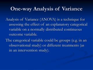
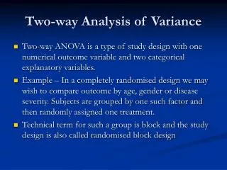
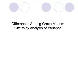
1 Way Analysis of Variance (ANOVA) Peter Shaw RU

1 way ANOVA – What is it? • This is a parametric test, examining whether the means differ between 2 or more populations. Females Males Site 2 Site 3 Site 1 Do males differ from females? Do results differ between these sites?

This is not in itself so unusual, indeed we are spoiled for choice:

So why am I spending so much time on anova? 1: Because anova is the definitive analytical tool: it allows one to ask questions that cannot be asked any other way. 2: You need to be familiar with the layout of anova tables. 3: Because I want you to understand the degrees of freedom associated with anova models. There are deep pitfalls associated with allocation of dfs, and inspection of the dfs in an anova table allow one to understand immediately what model another researcher has used.

What anova actually does: • It partitions the variation in the data into components, some of which can be explained by the experimenter (such as the difference between two treatments), and some of which is unexplained. • The unexplained variation is called “error”, but is in fact essential to performing the anova. It generates a test statistic F, which is the ratio of explained to unexplained variation. This can be thought of as a signal:noise ratio. Thus large values of F indicate a high degree of pattern within the data and imply rejection of H0. It is thus similar to the t test - in fact ANOVA on 2 groups is equivalent to a t test [F = t2 ; formally F 1,n-2 = (Tn-2)2]

The core of anova is to partition the sum of squares of a dataset: This is the summed values of (X-mean) 2, otherwise known as the sum of residuals2. Value Residuals Overall mean (μ) 1 2 3 4 5 6 7 8 Datapoint number Linear model: Each observation is the mean plus a random error Xi =μ + ei Total sum of squares = SStot= Σi (Xi-mean) 2 = Σi (ei * ei)

Now we split the data up into treatments: New residuals Overall mean (μ) Mean of treatment 2 1 2 3 4 5 6 7 8 Datapoint number Treatment 1 Treatment 2 Linear model: Each observation is the mean plus a treatment effect plus random error: Xti =μ +Tt+ eti Total sum of squares = Σi (Xi- μ) 2 = Σti (eti * eti) + Σti (Tti * Tti) = error sum of squares + treatment sum of squares (This is how variation is partitioned. Notice that it only works if Σti (eti) = Σti (Tti) = 0)

Now we have one sum of squares which has been partitioned into two sources, explained and unexplained. The null hypothesis H0 says that these two sources of variation should be equally unimportant, both unexplained random noise. In order to test this we cannot simply look at the sums of squares (because the more samples you collect the more variation you may find), but first divide these by their degrees of freedom to convert SS into variance: Total variance = total SS / total df – true but not used in most anova tables treatment variance = treatment SS / treatment df error variance = error SS / error df. F ratio (signal/noise) = treatment variance /error variance.

Exact layout varies somewhat - I dislike SPSS’s version! Anova tables: Learn this layout parrot-fashion! It is correct for a 1-way anova with N observations and T treatments. Source df SS MS F treatment (T-1) SStrt =SStrt/(T-1) MStrt/MSerr error…………by subtraction Sserr =SSerr/dferr Total (N-1) Finally, you (or the PC) consult tables or otherwise obtain a probability of obtaining this F value given dfs for treatment and error.

It is formally possible to perform an anova by calculating the values of treatment and error for each observation in turn – I have a handout showing this. In practice no-one does it this way because there is a labour-saving shortcut that is easily learned and implemented, which I intend to show you now.

How to do an ANOVA by hand: 1: Calculate N, Σx, Σx2 for the whole dataset. 2: Find the Correction factor CF = (Σx * Σx)/N 3: Find the total Sum of Squares for the data = Σ(xi2)– CF 4: add up the totals for each treatment in turn (Xt.), then calculate Treatment Sum of Squares SStrt = Σt(Xt.*Xt.)/r - CF where Xt. = sum of all values within treatment t, and r is the number of observations that went into that total. 3: Draw up ANOVA table, getting error terms by subtraction.

One way ANOVA’s limitations • This technique is only applicable when there is one treatment used. • Note that the one treatment can be at 3, 4,… many levels. Thus fertiliser trials with 10 concentrations of fertiliser could be analysed this way, but a trial of BOTH fertiliser and insecticide could not.

Class data – your turn T1 T2 T3 7 14 20 8 16 18 11 19 22 15 18 19 12 15 16 Totals (to be nice to you!) 53 82 95

What to do when you want to test : H0: group means are the same When the data are clearly not normally distributed? If you have 2 groups, you can fall back on Mann-Whitney’s U test BUT: 3 or more groups – you can’t do multiple U tests, just as you can’t do multiple t tests in place of a 1-way anova. (Why not?) There are 2 good alternatives, one of which is supplied in SPSS, one of which needs special code (I have some home-written). 1: Kruskal-Wallis non-parametric anova (good and safe) 2: use normal anova but use a Monte-Carlo approach to empirically estimate p values. (This is a perfect, safe and reliable way to generate p values, but is not widely available).

Post-hoc tests Often one runs an ANOVA on a dataset where the “treatment” variable comes at >3 levels. If p>0.05 you simply assume that the groups do not differ. If however p<0.05, students often ask whether this proves some specific difference, such as showing that site 1 differs from site 2. The simple answer is “NO”. The p value tests the classification as a whole, and you can’t infer specific differences from it. If you do want to ask about a specific division within your classification you need to explore the world of post-hoc tests (=”after the event”). There are a plethora of these, and you can run them by hand, but you need to be careful of handling your significance levels.

Why you don’t do multiple t tests. Or any other test, unless you have your eyes open…. Take random data and assemble into 2 piles, then test H0: no difference between them. Using p = 0.05 you know that you will reject this H0 1 time in 20. That is what p = 0.05 means. hat Now assemble into 3 piles, then test H0: no difference between teach pair: P1-P2, P1-P3, P2-P3 1 time in 20 p1-p2 is * 1 time in 20 p1-p3 is * 1 time in 20 p2-p3 is * hat p1 p2 p3

Now we ask what the probability is that we will end up accepting H0. This involves accepting H0 in test 1 (P1P2), AND in P1-P3, AND in P2P3. In each case the probability of accepting H0 is 0.95 (=1-p), but the probability of accepting the 3 together is 0.95*0.95*0.95 = 0.857375 (nearly, but not quite, 1-3*p). But if p(accepting H0) = 0.86, then p(rejecting H0) = 0.14. So in random data you will reject H0 1 time in 7, not 1 in 20. So if you claim in your write-up that you used p=0.05 you are lying, albeit probably unwittingly. It is OK to do this PROVIDING you know what you are doing, and you apply a more stringent criterion to each individual test. If you are doing N different tests on subsets of the same data, each one should run at a significance level of P = 1-(1-α)1/N = 1- n (1- α) Where α is the final significance level. 3 tests, α = 0.05, adjusted p = 1-0.95^(1/3) = 0.017.

Are hidden under “Compare means – 1 way anova”. Post-hoc tests in SPSS

Dissolved Fe in water draining Pelenna mine, Swansea. F6,49 = 72.9 p<0.001 But which sites differ from each other? Fe, ppm

Duncan’s multiple range test: Note 1: Means are sorted into ascending order 2: all bar 2 are in a homogenous subgroup: site 3 is in a group by itself, as is site 2.

Presentation methods:1: Leave means sorted into order and underline those that do not differ A B C • 7 6 5 4 3 2 • Site

2: the ABC method Leave the means in their original order but indicate which group they are in by giving a letter of the alphabet to each line in the graph just presented. Then you add the text “means followed by the same letter do not differ at p<0.05”. A C B A A A A

And if the data are very non-normal? You have always got a non-parametric anova, known as the Kruskal Wallis test. This does not have a post-hoc test, but you can create one with care. 1: Compare every group with every other by a U or K-W test, but apply a more stringent significance test as explained earlier. 2: Sort means (or better medians) into ascending order, and underline those which do not differ significantly as before.

Mayflies on Pelenna stream (4 sites only). P<0.05 by Kruskal-Wallis test. P values for each pairwise comparison in turn:

Adjust significance to 1-(0.95^1/6) = 0.0085, and underline sites that do not differ at this level B A 2 1 3 4 Site Or list as follows: Site 1AB 2A 3AB 4B

1 Way Analysis of Variance (ANOVA)