Local and Stochastic Search
460 likes | 607 Vues
Local and Stochastic Search. Based on Russ Greiner’s notes. A Different Approach. So far: systematic exploration: Explore full search space (possibly) using principled pruning (A*, . . . ) Best such algorithms (IDA*) can handle

Local and Stochastic Search
E N D
Presentation Transcript
Local and Stochastic Search Based on Russ Greiner’s notes
A Different Approach • So far: systematic exploration: • Explore full search space (possibly) using principled pruning (A*, . . . ) • Best such algorithms (IDA*) can handle • 10100 states ≈ 500 binary-valued variables (ballpark figures only!) • but. . . some real-world problem have 10,000 to 100,000 variables 1030,000 states • We need a completely different approach: • Local Search Methods or • Iterative Improvement Methods
Local Search Methods • Applicable when seeking Goal State & don't care how to get there. E.g., • N-queens, map coloring, . . . • VLSI layout, planning, scheduling, TSP, time-tabling, . . . • Many (most?) real Operations Research problems are solved using local search!
Random Search • Select (random) initial state (initial guess at solution) • Make local modification to improve current state • Repeat Step 2 until goal state found (or out of time) Requirements: • generate a random (probably-not-optimal) guess • evaluate quality of guess • move to other states (well-defined neighborhood function) . . . and do these operations quickly. . .
Example: 4 Queen • States: 4 queens in 4 columns (256 states) • Operators: move queen in column • Goal test: no attacks • Evaluation: h(n) = number of attacks
Example: Graph Coloring • Start with random coloring of nodes • Change color of one node to reduce # of conflict • Repeat 2
Problems with Hill Climbing • Foothills / Local Optimal: No neighbor is better, but not at global optimum. • (Maze: may have to move AWAY from goal to find (best) solution) • Plateaus: All neighbors look the same. • (8-puzzle: perhaps no action will change # of tiles out of place) • Ridges: going through a sequence of local maxima • Ignorance of the peak: Am I done?
Hill-climbing search: 8-queens problem • A local minimum with h = 1
Issues The Goal is to find GLOBAL optimum. • How to avoid LOCAL optima? • How long to do plateau walk? • When to stop? • Climb down hill? When?
Overcoming Local Optimum and Plateau • Random restarts • Simulated annealing • Mixed-in random walk • Tabu search (prevent repeated states) • Others (Genetic algorithms/programming, . . . )
Local Search Example: SAT(Russell & Norvig p221-225) • Many real-world problems can be translated into propositional logic (A v B v C) ^ (¬B v C v D) ^ (A v ¬C v D) . . . solved by finding truth assignment to variables (A, B, C, . . . ) that satisfies the formula • Applications • planning and scheduling • circuit diagnosis and synthesis • deductive reasoning • software testing • . . .
Satisfiability Testing • Best-known systematic method: • Davis-Putnam Procedure (1960) • Backtracking depth-first search (DFS) through space of truth assignments (with unit-propagation)
Greedy Local Search: GSAT • GSAT: 1. Guess a random truth assignment 2. Flip value assigned to the variable that yields the largest increase of the total # of satisfied clauses. (Note: Flip even if the increase is 0, but not negative) 3. Repeat until all clauses satisfied, or have performed “enough” flips 4. If no sat-assign found, repeat entire process, starting from a different initial random assignment.
Systematic vs. Stochastic • Systematic search: • DP systematically checks all possible assignments. • Can determine if the formula is unsatisfiable. • Stochastic search: • Guided random search approach. • Once we find it, we're done. • Can't determine unsatisfiability.
What Makes a SAT Problem Hard? • Suppose we have n variables to write m clauses with k variables each. • We negate the resulting variables randomly (flip an unbiased coin). • What is the number of possible sentences in terms of n, m, and k ? • What if there are many variables and only a smaller number of clauses? • What if there are many clauses and only a smaller number of variables?
Phase Transition • For 3-SAT • m/n < 4.2, under constrained: nearly all sentences sat. • m/n > 4.3, over constrained: nearly all sentences unsat. • m/n ~ 4.26, critically constrained: need to search
Phase Transition • Under-constrained problems are easy, just guess an assignment. • Over-constrained problems are easy, just say “unsatisfiable” (often easy to verify using Davis-Putnam). • At a m/n ratio of around 4.26, there is a phase transition between these two different types of easy problems. This transition sharpens as n increases. • For large n, hard problems are extremely rare (in some sense).
Improvements to Basic Local Search • Issue: • How to move more quickly to successively better plateaus? • Avoid “getting stuck” / local maxima? • Idea: Introduce uphill moves (“noise”) to escape from plateaus/local maxima • Noise strategies: 1. Simulated Annealing • Kirkpatrick et al. 1982; Metropolis et al. 1953 2. Mixed Random Walk • Selman and Kautz 1993
Simulated Annealing • Pick a random variable If flip improves assignment: do it. Else flip with probability p = e-δ/T = 1/(eδ/T ) • δ = # of additional clauses becoming unsatisfied • T = “temperature” • Higher temperature = greater chance of wrong-way move • Slowly decrease T from high temperature to near 0. • Q: What is p as T tends to infinity? . . . as T tends to 0? For δ = 0? • Thus, bad moves likely to be allowed at the start when T is high.
Notes on SA • Noise model based on statistical mechanics • . . . introduced as analogue to physical process of growing crystals • Kirkpatrick et al. 1982; Metropolis et al. 1953 • Convergence: • 1. W/ exponential schedule, will converge to global optimum • 2. No more-precise convergence rate (Recent work on rapidly mixing Markov chains) • Key aspect: upwards / sideways moves • Expensive, but (if have enough time) can be best • Hundreds of papers/ year; • Many applications: VLSI layout, factory scheduling, . . .
Properties of simulated annealing search • One can prove: If T decreases slowly enough, then simulated annealing search will find a global optimum with probability approaching 1 • Widely used in VLSI layout, airline scheduling, etc
Local Beam Search • Keep track of k states rather than just one • Start with k randomly generated states • At each iteration, all the successors of all k states are generated • If any one is a goal state, stop; else select the k best successors from the complete list and repeat.
Pure WalkSat • PureWalkSat( formula ) Guess initial assignment While unsatisfied do Select unsatisfied clause c = ±Xi v ±Xj v ±Xk Select variable v in unsatisfied clause c Flip v
Mixing Random Walk with Greedy Local Search • Usual issues: • Termination conditions • Multiple restarts • Value of p determined empirically, by finding best setting for problem class
Finding the best value of p • WalkSat[p]: • W/prob p, flip var in unsatisfied clause • W/prob 1-p, make a greedy flip to minimize # of unsatisfied clauses • Q: What value for p? • Let: Q[p, c] be quality of using WalkSat[p] on problem c. • Q[p, c] = Time to return answer, or = 1 if WalkSat[p] return (correct) answer within 5 minutes and 0 otherwise, or = . . . perhaps some combination of both . . . • Then, find p that maximize the average performance of WalkSat[p] on a set of challenge problems.
Experimental Results: Hard Random 3CNF • Time in seconds • Effectiveness: prob. that random initial assignment leads to a solution. • Complete methods, such as DP, up to 400 variables • Mixed Walk better than Simulated Annealing • better than Basic GSAT • better than Davis-Putnam
Overcoming Local Optimum and Plateau • Random restarts • Simulated annealing • Mixed-in random walk • Tabu search (prevent repeated states) • Others (Genetic algorithms/programming, . . . )
Other Techniques • random restarts: restart at new random state after pre-defined # of local steps. • [Done by GSAT] • tabu: prevent returning quickly to same state. • Implement: Keep fixed length queue (tabu list). • Add most recent step to queue; drop oldest step. • Never make step that's on current tabu list. • Example: • without tabu: • flip v1, v2, v4, v2, v10, v11, v1, v10, v3, ... • with tabu (length 5)—possible sequence: • flip v1, v2, v4, v10, v11, v1, v3, ... • Tabu very powerful; competitive w/ simulated annealing or random walk (depending on the domain)
Genetic Algorithms • A class of probabilistic optimization algorithms • A genetic algorithm maintains a population of candidate solutions for the problem at hand, and makes it evolve by iteratively applying a set of stochastic operators • Inspired by the biological evolution process • Uses concepts of “Natural Selection” and “Genetic Inheritance” (Darwin 1859) • Originally developed by John Holland (1975)
The Algorithm • Randomly generate an initial population. • Select parents and “reproduce” the next generation • Evaluate the fitness of the new generation • Replace the old generation with the new generation • Repeat step 2 though 4 till iteration N
Stochastic Operators • Cross-over • decomposes two distinct solutions and then randomly mixes their parts to form novel solutions • Mutation • randomly perturbs a candidate solution
Genetic Algorithm Operators Mutation and Crossover 1 0 1 0 1 1 1 Parent 1 1 1 0 0 0 1 1 Parent 2 1 0 1 0 0 1 1 Child 1 Mutation Child 2 1 1 0 0 1 1 0
Examples: Recipe • To find optimal quantity of three major ingredients (sugar, wine, sesame oil) denoting ounces. • Use an alphabet of 1-9 denoting ounces.. • Solutions might be 1-1-1, 2-1-4, 3-3-1.
Examples • Mutation: The recipe example: 1-2-3 may be changed to 1-3-3 or 3-2-3. • Parameters to adjust • How often? • How many digits change? • How big?
More examples: • Crossover Recipe : Parents 1-3-3 & 3-2-3. Crossover point after the first digit. Generate two offspring: 3-3-3 and 1-2-3. Can have one or two point crossover.
Randomized Algorithms • A randomized algorithm is defined as an algorithm where at least one decision is based on a random choice.
Monte Carlo and Las Vegas There are two kinds of randomized algorithms: • Las Vegas: A Las Vegas algorithm always produces the correct answer, but randomness only influence the resources used. E.g. Randomized Quiksort with pivot randomly chosen. • Monte Carlo: A Monte Carlo algorithm runs for a fixed number of steps for each input and produces an answer that is correct with a bounded probability
Local Search Summary • Surprisingly efficient search technique • Wide range of applications • Formal properties elusive • Intuitive explanation: • Search spaces are too large for systematic search anyway. . . • Area will most likely continue to thrive
