Download
1 / 12
120 likes | 243 Vues
Fractal tools for the analysis of star-forming regions. Néstor Sánchez Emilio J. Alfaro Enrique Pérez Instituto de Astrofísica de Andalucía, Graná , Spain. V Workshop "Estallidos", Granada, 2007. Introduction / Motivation. ↑. Star formation process. Initial conditions: ISM structure

E N D
Fractal tools for the analysisof star-forming regions Néstor Sánchez Emilio J. Alfaro Enrique Pérez Instituto de Astrofísica de Andalucía, Graná , Spain V Workshop "Estallidos", Granada, 2007
Introduction / Motivation ↑ Star formation process. Initial conditions: ISM structure Objective/Systematic ISM characterization ISM structure vs environmental variables Our approach: ISM topology Fractal dimension (Df): degree of complexity (smoothness or clumpyness) of the ISM ↑ ↑ ↑ ↑
Fractal dimension estimators F ~ xDf Perimeter-area: P ~ ADper/2 Mass-radius: M ~ rDm Correlation integral: C ~ rDc Simulated Fractal Clouds Df=2.3 Df=2.6
Factors affecting theestimation of Df: • Opacity • Noise • Proyection effects • Image resolution 2D: Df_calcu < Df_theor Dper = Dper(Df,Npix) (Sanchez, Alfaro, Perez, ApJ, 2005)
Factors affecting theestimation of Df: • Opacity • Noise • Proyection effects • Image resolution tau_0 = 0 tau_0 = 1 tau_0 = 2 (Sanchez, Alfaro, Perez, ApJ, 2007)
Factors affecting theestimation of Df: • Opacity • Noise • Proyection effects • Image resolution Dper ≠ Dper(tau) (Sanchez, Alfaro, Perez, ApJ, 2007)
Factors affecting theestimation of Df: • Opacity • Noise • Proyection effects • Image resolution Contrast = I(max)/s.d.(background) Recipe: Smooth the image to maximizing the contrast (taken from Vogelaar & Wakker 1994) Dper_opt = Dper(max. cont.)
Application to emission maps Ophiuchus, Perseus (COMPLETE, Ridge et al. 2006) Orion (Nobeyama, Tatematsu et al. 1993) 13CO maps
Application to emission maps (Sanchez, Alfaro, Perez, ApJ, 2007) Df = 2.7 +/- 0.1 Df ~ 2.6 is roughly consistent with average observed properties (Sanchez, Alfaro, Perez, ApJ, 2006)
New-born stars • Df(ISM) ---> Df (star distribution) • Application to the Gould Belt (closest star formation complex): GB LGD Blue = O-B3 Red = B4-B6
Df - Gould Belt GB-early: Df = 2.68 +/- 0.04 GB-late: Df = 2.85 +/- 0.04 LGD-early: Df = 2.89 +/- 0.06 LGD-late: Df = 2.84 +/- 0.06 (Sanchez et al. 2007, in preparation)
Conclusions • Well-defined fractal clouds were simulated, various Df estimators analyzed, and different effects quantified by using "good" (modesty aside) algorithms. • Fractal analysis is a "reliable" tool for analysing both ISM (gas) structure and star distribution. • Df(ISM) ≈ 2.7 +/- 0.1 (> 2.3) (universal?) • Df GB-early = 2.68 +/- 0.04 (stars ↔ ISM?) • Df GB-late = 2.85 +/- 0.04 (Df increase with time?) • In the very, very near future (tomorrow?): distribution of star forming regions in galaxies, stars in clusters, etc.