Download
1 / 23
230 likes | 392 Vues
Scalable and Scalably-Verifiable Sequential Synthesis. Alan Mishchenko Mike Case Robert Brayton UC Berkeley. Overview. Introduction Computations SAT sweeping Induction Partitioning Verification Experiments Future work. Introduction. Combinational synthesis

E N D
Scalable and Scalably-Verifiable Sequential Synthesis Alan Mishchenko Mike Case Robert Brayton UC Berkeley
Overview • Introduction • Computations • SAT sweeping • Induction • Partitioning • Verification • Experiments • Future work
Introduction • Combinational synthesis • Cuts at the register boundary • Preserves state encoding, scan chains & test vectors • No sequential optimization – easy to verify • Sequential synthesis • Runs retiming, re-encoding, use of sequential don’t-cares, etc • Changes state encoding, invalidates scan chains & test vectors • Some degree of sequential optimization – non-trivial to verify • Scalably-verifiable sequential synthesis • Merges sequentially equivalent registers and internal nodes • Minor change to state encoding, scan chains & test vectors • Some degree of sequential optimization – easy to verify!
? SAT Applying SAT to the output ? ? ? SAT-2 SAT-1 C D B SAT-3 A Proving internal equivalences in a topological order Combinational SAT Sweeping • Naïve CEC approach – SAT solving • Build output miter and call SAT • works well for many easy problems • Better CEC approach – SAT sweeping • based on incremental SAT solving • Detects possibly equivalent nodes using simulation • Candidate constant nodes • Candidate equivalent nodes • Runs SAT on the intermediate miters in a topological order • Refines the candidates using counterexamples
Sequential SAT Sweeping • Sequential SAT sweeping is similar to combinational one in that it detects node equivalences • The difference is, the equivalences are sequential • They hold only in the reachable state space • Every comb. equivalence is a seq. one, not vice versa • It makes sense to run comb. SAT sweeping beforehand • Sequential equivalence is proved by K-step induction • Base case • Inductive case • Efficient implementation of induction is key!
SAT-1 SAT-1 SAT-3 A A A B B B SAT-4 SAT-2 SAT-2 C C C D D D Base Case Inductive Case ? Candidate equivalences: {A,B}, {C,D} ? Proving internal equivalences in a topological order in frame K ? ? PIk 0 0 PI1 C ? D A Assuming internal equivalences to in uninitialized frames 0 through K-1 ? B PI1 0 0 PI0 C D Initial state A B Proving internal equivalences in initialized frames 0 through K-1 PI0 Symbolic state
Efficient Implementation • Two observations: • Both base and inductive cases of K-step induction are runs of combinational SAT sweeping • Tricks and know-hows of combinational sweeping are applicable • The same integrated package can be used • Starts with simulation • Performs node checking in a topological order • Benefits from the counter-example simulation • Speculative reduction • Has to do with how the assumptions are made (see next slide)
Speculative Reduction • Inputs to the inductive case • Sequential circuit • The number of frames to unroll (K) • Candidate equivalence classes • One node in each class is designated as the representative node • Currently the representatives are the first nodes in a topological order • Speculative reduction moves fanouts to the representative nodes • Makes 80% of the constraints redundant • Dramatically simplifies the resulting timeframes (observed 3x reductions) • Leads to saving 100-1000x in runtime during incremental SAT solving 0 0 A A B B Adding assumptions with speculative reduction Adding assumptions without speculative reduction
Partitioning for Induction • A simple output-partitioning algorithm was implemented • One person-day of programming • CEC and induction became more scalable • Typical reduction in runtime is 20x for a 1M-gate design • Partitioning is meant to make SAT problems smaller • The same partitioning is useful for parallelization! • Partitioning algorithm • Pre-processing: For all POs, finds PIs they depend on • Main loop: For each PO, in a degreasing order of support size • Finds a partition by looking at the supports • Chooses partition with min linear combination of attraction and repulsion (determined by the number of common and new variables in this PO) • Imposes restrictions on the partition size • Post-processing: Compacts smaller partitions • Complexity: O( numPis(AIG) * numPos(AIG) )
? A’ = B’ C = D A = B ? C’ D’ A’ B’ C’ = D’ One timeframe of the design C D A B C = D A = B Partitioning Details • Currently induction is partitioned only for register correspondence • In this case, it is enough to partition only one timeframe! • In each iteration of induction • The design is re-partitioned • Nodes in each candidate equiv class are added to the same partition • Constant candidates can be added to any partition • Candidates are merged at the PIs and proved at the POs • After proving all partitions, the classes are refined • The partitioned induction has the same fixed-point as the monolithic induction while the number of iterations can differ (different c-examples lead to different refinements) Partition 1 Illustration for two cand equiv classes: {A,B}, {C,D} Partition 2
Other Observations • Surprisingly, the following are found to be of little or no importance for speeding up the inductive prover • The quality of initial equivalence classes • How much simulation (semi-formal filtering) was applied • AIG rewriting on speculated timeframes • Although AIG can be reduced 20%, incremental SAT runs the same • The quality of AIG-to-CNF conversion • Naïve conversion (1 AIG node = 3 clauses) works just fine • Open question: Given these observations, how to speed up this type of incremental SAT?
N1 X … M N2 N1 X X Verification after PSS • Poison and antidote are the same! • The same inductive prover is used • during synthesis – to prove seq equivalence of registers and nodes • during verification – to prove seq equivalence of registers, nodes, and POs of two circuits • Verification is “unbounded” and “general-case” • No limit on the input sequence is imposed (unlike BMC) • No information about synthesis is passed to the verification tool • The runtimes of synthesis and verification are comparable • Scales to 10K-register designs – due to partitioning for induction Synthesis problem Equivalence checking problem
Integrated SEC Flow • The following is the sequence of transformations currently applied by the integrated SEC in ABC (command “dsec”) • creating sequential miter (“miter -c”) • PIs/POs are paired by name; if some registers have don’t-care init values, they are converted by adding new PIs and muxes; all logic is represented in the form of an AIG • sequential sweep (“scl”) • removes logic that does not fanout into POs • structural register sweep (“scl -l”) • removes stuck-at-constant and combinationally-equivalent registers • most forward retiming (“retime –M 1”) (disabled by switch “–r”, e.g. “dsec –r”) • moves all registers forward and computes new initial state • partitioned register correspondence (“lcorr”) • merges sequential equivalent registers (completely solves SEC after retiming) • combinational SAT sweeping (“fraig”) • merges combinational equivalent nodes before running signal correspondence • for ( K = 1; K 16; K = K * 2 ) • signal correspondence(“ssw”) // merges seq equivalent signals by K-step induction • AIG rewriting(“drw”) // minimizes and restructures combinational logic • most forward retiming // moves registers forward after logic restructuring • sequential AIG simulation // targets satisfiable SAT instances • post-processing (“write_aiger”) • if sequential miter is still unsolved, dumps it into a file for future use
Example of PSS in ABC abc 01> r iscas/blif/s38417.blif// reads in an ISCAS’89 benchmark abc 02> st; ps// shows the AIG statistics after structural hashing s38417 : i/o = 28/ 106 lat = 1636 and = 9238 (exor = 178) lev = 31 abc 03> ssw –K 1 -v // performs one round of signal correspondence using simple induction Initial fraiging time = 0.27 sec Simulating 9096 AIG nodes for 32 cycles ... Time = 0.06 sec Original AIG = 9096. Init 2 frames = 84. Fraig = 82. Time = 0.01 sec Before BMC: Const = 5031. Class = 430. Lit = 9173. After BMC: Const = 5031. Class = 430. Lit = 9173. 0 : Const = 5031. Class = 430. L = 9173. LR = 1928. NR = 3140. 1 : Const = 4883. Class = 479. L = 8964. LR = 1554. NR = 2978. … 28 : Const = 145. Class = 177. L = 756. LR = 198. NR = 9099. 29 : Const = 145. Class = 176. L = 753. LR = 195. NR = 9090. SimWord = 1. Round = 2025. Mem = 0.38 Mb. LitBeg = 9173. LitEnd = 753. ( 8.21 %). Proof = 5022. Cex = 2025. Fail = 0. FailReal = 0. C-lim = 10000000. ImpRatio = 0.00 % NBeg = 9096. NEnd = 8213. (Gain = 9.71 %). RBeg = 1636. REnd = 1345. (Gain = 17.79 %). AIG simulation = 2.25 sec AIG traversal = 0.01 sec SAT solving = 3.71 sec Unsat = 0.16 sec Sat = 3.55 sec Fail = 0.00 sec Class refining = 0.38 sec TOTAL RUNTIME = 8.51 sec abc 04> ps// shows the AIG statistics after merging equivalent registers and nodes s38417 : i/o = 28/ 106 lat = 1345 and = 8213 (exor = 116) lev = 31 abc 04> dsec –r// runs the unbounded SEC on the resulting network against the original one Networks are equivalent. Time = 15.59 sec
Experimental Results • Public benchmarks • 25 test cases • ITC’99 (b14, b15, b17, b20, b21, b22) • ISCAS’89 (s13207, s35932, s38417, s38584) • IWLS’05(systemcaes, systemcdes, tv80, usb_funct, vga_lcd, wb_conmax, wb_dma, ac97_ctrl, aes_core, des_area, des_perf, ethernet, i2c, mem_ctrl, pci_spoci_ctrl) • Industrial benchmarks • 50 test cases • Nothing else is known • Workstation • Intel Xeon 2-CPU 4-core, 8Gb RAM
ABC Scripts • Baseline • choice;if; choice;if; choice;if // comb synthesis and mapping • Register correspondence (Reg Corr) • scl –l // structural register sweep • lcorr // register correspondence using partitioned induction • dsec –r // SEC • choice;if; choice;if; choice;if // comb synthesis and mapping • Signal correspondence (Sig Corr) • scl –l // structural register sweep • lcorr // register correspondence using partitioned induction • ssw // signal correspondence using non-partitioned induction • dsec –r // SEC • choice;if; choice;if; choice;if // comb synthesis and mapping
Public Benchmarks Columns “Baseline”, “Reg Corr” and “Sig Corr” show geometric means.
Industrial Benchmarks In case of multiple clock domains, optimization was applied only to the domain with the largest number of registers.
Future • Continue tuning for scalability • Speculative reduction • Partitioning • Experiment with new ideas • Unique-state constraints • Interpolate when induction fails • Synthesizing equivalence • Go beyond merging sequential equivalences • Add logic restructuring using subsets of unreachable states • Add retiming (improves delay on top of reg/area reductions) • Add iteration (led to improvements in other synthesis projects) • etc