Download
1 / 14
150 likes | 192 Vues
Learn about parameterizing vertical mixing processes in the coastal ocean using advanced closure schemes and boundary layer parameterizations. Model setups, circulation models, and diffusivity profiles are explored based on pioneering research.

E N D
Parameterizing Vertical Mixing in the Coastal Ocean Scott Durski, Scott Glenn, Dale Haidvogel, Hernan Arango • Institute of Marine and Coastal Sciences • Rutgers University • New Brunswick, NJ • January 27, 1999
u Kv ku*z u* Vertical Mixing Processes Model Parameterizations 2nd and higher order closure schemes - Mellor-Yamada, Gaspar, Stull. Boundary layer mixing K profile parameterizations (1st order) - Troen and Mahrt, Large, McWilliams and Doney. ~ Mixed layer models - Price et al. ,Kraus and Turner. Langmuir circulation Surface wave breaking Interior shear driven processes Gradient Richardson number based schemes - Pacanowski-Philander, Large et. al(interior scheme), Kantha and Clayson. 2nd and higher order closure schemes - Mellor-Yamada, Gaspar, Stull. Background mixing constant - Large et al. Internal wave breaking Proportional to N-1 - Gargett and Holloway.. Double diffusive processes Density ratio base schemes - Large et al.
Large, McWilliams and Doney, K-Profile parameterization Ko 0.5 Rig Boundary layer mixing Interior mixing Mixing parameterized as a function of boundary layer depth, turbulent velocity scale and a dimensionless ‘shape’ function. Shear generated mixing Based on gradient Richardson Number Boundary layer depth Based on bulk Richardson number. Internal wave mixing Constant ‘background’ mixing value from open ocean thermocline observations. Turbulent velocity scale From atmospheric surface boundary layer similarity theory Double diffusive mixing Based on laboratory measurements, based on density ratio. Shape function Third order polynomial with coefficients determined from boundary conditions at surface and ocean ‘interior’.
? ? ? ? ? Modifications to the K-profile Parameterization for coastal ocean application. Addition of a bottom boundary layer parameterization 1) Matching with log layer similarity theory where surface boundary layer extends to the bottom.. 2) Apply matching rules when surface and bottom boundary layers overlap. 3) Add a K-profile parameterization for the bottom boundary layer modeled after SBL approximation. Kv = ku*z Change in internal wave mixing parameterization for interior Replace constant value with the buoyancy frequency dependent formulation of Gargett and Holloway Kvi = 1.0x10e-7 N-1
2-Dimensional Model Setup Circulation model • S-coordinate Rutgers University Model (SCRUM). Idealized 2-dimensional domain 21.5 • 75 km horizontal extent. • depth ranges from 6m at the coast to 40m offshore. • Grid resolution varies from 500m at the coast to 4km offshore. • 50 sigma coordinate vertical levels. • open boundary conditions applied at offshore boundary. 20.6 19.6 Initialization 18.7 • horizontally uniform stratification. • stratification ranging from 1017.8 kg/m3 to 1021.5 kg/m3 . 17.8 Forcing • 4 days of uniform 0.28 dyne along-shore upwelling favorable wind stress.
Density Across-shore velocity Along-shore velocity Basic Model Response • Advectively dominated upwelling process. • Formation of an alongshore jet reaching a magnitude of 50 cm/s • Development of surface and bottom boundary layers • Vertical mixing ‘overcomes’ upwelling in the nearshore region before sub-pycnocline water reaches the coast
Model-Model Comparison The basic response with the two schemes is quite similar but .... • More intermediate density water is trapped at the coast with the Mellor-Yamada scheme. • The surface jet is approximately 10 cm/s weaker with the Mellor-Yamada scheme. Density Across-shore velocity Along-shore velocity LMD M-Y
The development of the upwelling front 1) The Mellor-Yamada parameterization entrains more water into the bottom boundary layer as the pycnocline advects shoreward causing the isopycnals of the bottom front to broaden 2)As a consequence of this weaker stratification occurs sooner in the near shore region with the Mellor - Yamada scheme. 3) Vertical mixing breaks down this weaker stratification forming a surface-to--bottom boundary layer earlier. This prevents further upwelling at the coast. Diffusivity LMD M-Y
M-Y LMD spreads isopycnals compresses isopycnals M-Y smaller LMD larger What causes the Mellor-Yamada scheme to entrain more? Diffusivity profiles 1) The gradient in diffusivity coefficient at the edge of the pycnocline tends to be greater with the LMD parameterization. 2) The higher stratification formed by the compression of isopycnals, creates an increasingly intense barrier to vertical mixing 3) Mixing at the base of the boundary layer in open ocean settings is likely to be characterized by significantly weaker gradients in diffusivity and density.
LMD Ko PP (1 + 5Ri)2 diffusivity Gradient Richardson number An alternate formulation for shear generated mixing 1) The Pacanowski and Philander parameterization estimates a more gradual variation of diffusivity with gradient Richardson number between Ri=0.15 and 0.6. Interior shear mixing formulations LMD PP K =
Comparison of original LMD shear mixing scheme with modified P-P interior. Using the Pacanowski and Philander shear mixing term for the interior produces frontal intensity and near shore densty structure more similar to the Mellor - Yamada scheme. Original LMD LMD w/PP interior
The development of the upwelling front Diffusivity LMD w/PP interior Original LMD
The modifications to the Large, McWilliams and Doney scheme produce a parameterization with behavior quite similar to the Mellor -Yamada scheme for a wind driven continental shelf upwelling simulation. • Greater entrainment into the bottom boundary layer produced by the Mellor -Yamada scheme leads to the formation of a less intense upwelling front and the trapping of more intermeadiate density water at the coast. • The greater entrainment by the Mellor-Yamada scheme is due to a weaker gradient in the diffusivity coefficient where the boundary layer meets the pycnocline. • More observations of mixing at the entrainment depth will help direct future model improvement. Summary