Chapter 2: Modeling Distributions of Data
180 likes | 207 Vues
Learn about describing location, percentiles, z-scores, cumulative frequency graphs, and density curves in statistical distributions.

Chapter 2: Modeling Distributions of Data
E N D
Presentation Transcript
Chapter 2: Modeling Distributions of Data Section 2.1 Describing Location in a Distribution The Practice of Statistics, 4th edition - For AP* STARNES, YATES, MOORE
Chapter 2Modeling Distributions of Data • 2.1Describing Location in a Distribution • 2.2Normal Distributions
Brainteaser • As oou oan oee, oy poinoer oepoacos eoero thord oetoer oito tho leoteo 'o'.How mony oifoeront oetoero haoe boen oepoacod? • Answer: 15.The sentences should read:As you can see, my printer replaces every third letter with the letter 'o'.How many different letters have been replaced?
Section 2.1Describing Location in a Distribution Learning Objectives After this section, you should be able to… • MEASURE position using percentiles • INTERPRET cumulative relative frequency graphs • MEASURE position using z-scores • TRANSFORM data • DEFINE and DESCRIBE density curves
Describing Location in a Distribution • Measuring Position: Percentiles • One way to describe the location of a value in a distribution is to tell what percent of observations are less than it. Definition: The pth percentile of a distribution is the value with p percent of the observations less than it. Jenny earned a score of 86 on her test. How did she perform relative to the rest of the class? 6 7 7 2334 7 5777899 8 00123334 8 569 9 03 6 7 7 2334 7 5777899 8 00123334 8 569 9 03 Her score was greater than 21 of the 25 observations. Since 21 of the 25, or 84%, of the scores are below hers, Jenny is at the 84th percentile in the class’s test score distribution.
Describing Location in a Distribution • Cumulative Relative Frequency Graphs A cumulative relative frequency graph (or ogive) displays the cumulative relative frequency of each class of a frequency distribution.
Interpreting Cumulative Relative Frequency Graphs Describing Location in a Distribution Use the graph from page 88 to answer the following questions. • Was Barack Obama, who was inaugurated at age 47, unusually young? • Estimate and interpret the 65th percentile of the distribution 65 11 58 47
Describing Location in a Distribution • Measuring Position: z-Scores • A z-score tells us how many standard deviations from the mean an observation falls, and in what direction. Definition: If x is an observation from a distribution that has known mean and standard deviation, the standardized value of x is: A standardized value is often called a z-score. Jenny earned a score of 86 on her test. The class mean is 80 and the standard deviation is 6.07. What is her standardized score?
Describing Location in a Distribution • Using z-scores for Comparison We can use z-scores to compare the position of individuals in different distributions. Jenny earned a score of 86 on her statistics test. The class mean was 80 and the standard deviation was 6.07. She earned a score of 82 on her chemistry test. The chemistry scores had a fairly symmetric distribution with a mean 76 and standard deviation of 4. On which test did Jenny perform better relative to the rest of her class?
Describing Location in a Distribution • Transforming Data Transforming converts the original observations from the original units of measurements to another scale. Transformations can affect the shape, center, and spread of a distribution. Effect of Adding (or Subracting) a Constant • Adding the same number a (either positive, zero, or negative) to each observation: • adds a to measures of center and location (mean, median, quartiles, percentiles), but • Does not change the shape of the distribution or measures of spread (range, IQR, standard deviation). Example, p. 93
Describing Location in a Distribution • Transforming Data Effect of Multiplying (or Dividing) by a Constant • Multiplying (or dividing) each observation by the same number b (positive, negative, or zero): • multiplies (divides) measures of center and location by b • multiplies (divides) measures of spread by |b|, but • does not change the shape of the distribution Example, p. 95
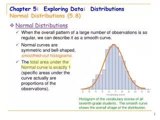
Describing Location in a Distribution • Density Curves • In Chapter 1, we developed a kit of graphical and numerical tools for describing distributions. Now, we’ll add one more step to the strategy. Exploring Quantitative Data • Always plot your data: make a graph. • Look for the overall pattern (shape, center, and spread) and for striking departures such as outliers. • Calculate a numerical summary to briefly describe center and spread. 4. Sometimes the overall pattern of a large number of observations is so regular that we can describe it by a smooth curve.
Describing Location in a Distribution • Density Curve • Definition: • A density curve is a curve that • is always on or above the horizontal axis, and • has area exactly 1 underneath it. • A density curve describes the overall pattern of a distribution. The area under the curve and above any interval of values on the horizontal axis is the proportion of all observations that fall in that interval. The overall pattern of this histogram of the scores of all 947 seventh-grade students in Gary, Indiana, on the vocabulary part of the Iowa Test of Basic Skills (ITBS) can be described by a smooth curve drawn through the tops of the bars.
Section 2.1Describing Location in a Distribution Summary In this section, we learned that… • There are two ways of describing an individual’s location within a distribution – the percentile and z-score. • A cumulative relative frequency graph allows us to examine location within a distribution. • It is common to transform data, especially when changing units of measurement. Transforming data can affect the shape, center, and spread of a distribution. • We can sometimes describe the overall pattern of a distribution by a density curve (an idealized description of a distribution that smooths out the irregularities in the actual data).
Looking Ahead… In the next Section… • We’ll learn about one particularly important class of density curves – the Normal Distributions • We’ll learn • The 68-95-99.7 Rule • The Standard Normal Distribution • Normal Distribution Calculations, and • Assessing Normality
When a clock's reflection is 2.30, what time is it really? 9:30
Can you complete this grid of letters. Each line is a valid 5 letter word with its first and last letter missing. • The missing letters form a word when read downwards and the same word appears both at the start and at the end. • What is the missing word? • *AGL* • *ABE* • *LUR* • *UTD* • *IDO*