Two-views geometry Outline

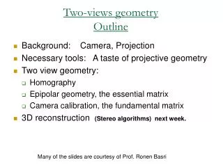
1. Two-views geometryOutline • Background: Camera, Projection • Necessary tools: A taste of projective geometry • Two view geometry: • Homography • Epipolar geometry, the essential matrix • Camera calibration, the fundamental matrix • 3D reconstruction (Stereo algorithms) next week. Many of the slides are courtesy of Prof. Ronen Basri

2. Objective 3-D Scene u’ u What can 2 images tell us about …. Faugeras et. al. ECCV 92

3. Objective 3-D Scene u’ u Study the mathematical relations between corresponding image points. “Corresponding”means originated from the same 3D point.

4. World Cup 66: England-Germany

5. World Cup 66: Second View

6. World Cup 66: England-Germany Conclusion: no goal (missing 3 inches) (Reid and Zisserman, “Goal-directed video metrology”)

7. Camera Obscura "Reinerus Gemma-Frisius, observed an eclipse of the sun at Louvain on January 24, 1544, and later he used this illustration of the event in his book De Radio Astronomica et Geometrica, 1545. It is thought to be the first published illustration of a camera obscura..." Hammond, John H., The Camera Obscura, A Chronicle

8. A few words about Cameras • Camera obscura dates from 15th century • First photograph on record shown in the book - 1822 • Basic abstraction is the pinhole camera • Current cameras contain a lens and a recording device (film, CCD, CMOS) • The human eye functions very much like a camera

9. Ideal Lenses Lens acts as a pinhole (for 3D points at the focal depth).

10. Regular Lenses E.g., the cameras in our lab. To learn more on lens-distortion see Hartley & Zisserman Sec. 7.4 p.189. Not part of this class.

11. Pinhole Camera

12. Single View Geometry ∏ f

13. Notation • O – Focal center • π – Image plane • Z – Optical axis • f – Focal length

14. Projection y x f Y X Z

15. Perspective Projection • Origin (0,0,0)is the Focal center • X,Y (x,y) axis are along the image axis (height / width). • Z is depth = distance along the Optical axis • f – Focal length

16. Orthographic Projection • Projection rays are parallel • Image plane is fronto-parallel • (orthogonal to rays) • Focal center at infinity

17. Scaled Orthographic Projection Also called “weak perspective”

18. Pros and Cons of Projection Models • Weak perspective has simpler math. • Accurate when object is small and distant. • Useful for object recognition. • Pinhole perspective much more accurate. • Used in structure from motion. • When accuracy really matters (SFM), we must model the real camera (exact imaging processes): • Perspective projection, calibration parameters (later), and all other issues (radial distortion).

19. Two-views geometryOutline • Background: Camera, Projection • Necessary tools: A taste of projective geometry • Two view geometry: • Homography • Epipolar geometry, the essential matrix • Camera calibration, the fundamental matrix • 3D reconstruction from two views (Stereo algorithms) Hartley & Zisserman: Sec. 2 Proj. Geom. of 2D. Sec. 3 Proj. Geom. of 3D.

20. Reading • Hartley & Zisserman: • Sec. 2 Proj. Geo. of 2D: • 2.1- 2.2.3 point lines in 2D • 2.3 -2.4 transformations • 2.7 line at infinity • Sec. 3 Proj. Geo. of 3D. • 3.1 – 3.2 point planes & lines. • 3.4 transformations

21. Why projective Geometry (Motivation) • Euclidean Geometry is good for questions like: what objects have the same shape (= congruent) Same shapes are related by rotation and translation

22. Why Projective Geometry (Motivation) • Answers the question what appearances (projections) represent the same shape Same shapes are related by a projective transformation

23. Why Projective Geometry (Motivation) Parallel lines meet at the horizon (“vanishing line”) Where do parallel lines meet?

24. Coordinates in Euclidean Space Not in space 0 1 2 3 ∞

25. Coordinates in Projective Line P1 Points on a line P1 are represented as rays from origin in 2D, Origin is excluded from space “Ideal point” k(1,1) k(0,1) k(-1,1) k(2,1) -1 0 1 2 ∞ k(1,0)

26. Coordinates in Projective Plane P2 Take R3 –{0,0,0} and look at scale equivalence class (rays/lines trough the origin). k(0,1,1) k(1,1,1) “Ideal point” k(0,0,1) k(1,0,1) k(x,y,0)

27. Projective Line vs. the Real Line “Ideal point” k(1,1) k(0,1) k(-1,1) k(2,1) -1 0 1 2 ∞ k(1,0)

28. k(0,1,1) k(1,1,1) “Ideal line” k(0,0,1) k(1,0,1) k(x,y,0) Projective Plane vs Euclidian plane

29. 2D Projective Geometry: Basics • A point: • A line: we denote a line with a 3-vector • Line coordinates are homogenous • Points and lines are dual: p is on l if • Intersection of two lines/points

30. Area of parallelogram bounded by u and v Cross Product Every entry is a determinant of the two other entries Hartley & Zisserman p. 581

31. Cross Product in matrix notation [ ]x Hartley & Zisserman p. 581

32. Example: Intersection of parallel lines Q: How many ideal points are there in P2? A: 1 degree of freedom family – the line at infinity

33. u’ u Projective Transformations

34. Transformations of the projective line Given a 2D linear transformation G:R2 R2 Study the induced transformation on the Equivalents classes. On the realization y=1 we get

35. Properties: • Invertible (T-1 exists) • Composable (To G is a projective transformation) • Closed under composition • Has 4 parameters • 3 degrees of freedom • Defined by 3 points Every point defines 1 constraint

36. Perspective mapping Pencil of rays Transformations of the projective line A perspective mapping is a projective transformation T:P1 P1 Perceptivity is a special projective mapping. Hartley & Zisserman p. 632 Lines connecting corresponding points are “concurrent”

37. Ideal points and projective transformations Projective transformation can map ∞ to a real point

38. Plane Perspective

39. 2D Projective Transformation 4 names 3 definitions • Projectivity: An invertible mapping h:P2 P2 S.T: • Homography. A 3x3 (non singular) invertible matrix acting on homogenous 3-vectores. • Collineation A transformations that map lines to lines Hartley & Zisserman p. 32

40. 2D Projective Transformation • H is defined up to scale • 9 parameters • 8 degrees of freedom • Determined by 4 corresponding points how does H operate on lines? Hartley & Zisserman p. 32

41. Plane Perspective This mapping clearly maps lines to lines

42. Plane Perspective acting on conics Hartley & Zisserman p. 30 & 36 Not part of this class

43. Hierarchy of Transformations Projective Affine Similarity Rigid (Isometry) Translation: Rotation: Scale Hartley & Zisserman p. Sec. 2.4

44. Euclidean Transformations (Isometries) Rotation: Translation:

45. Hierarchy of Transformations • Isometry (Euclidean), • Similarity, • Affine, general linear • Projective,

46. Invariants

47. Two-views geometryOutline • Background: Camera, Projection • Necessary tools: A taste of projective geometry • Two view geometry: • Homography • Epipolar geometry, the essential matrix • Camera calibration, the fundamental matrix • 3D reconstruction from two views (Stereo algorithms)

48. Two View Geometry • When a camera changes position and orientation, the scene moves rigidly relative to the camera 3-D Scene u’ u Rotation + translation

49. Objective: find formulas that links corresponding points 3-D Scene u’ u Rotation + translation

50. Two View Geometry (simple cases) • In two cases this results in homography: • Camera rotates around its focal point • The scene is planar Then: • Point correspondence forms 1:1mapping • depth cannot be recovered