Control Design for a DC Motor System
410 likes | 557 Vues
Explore design techniques and simulations for feedforward, feedback, and integral control of a DC motor system with compensators like proportional, lead, and PID. Compare controller designs and analyze system responses.

Control Design for a DC Motor System
E N D
Presentation Transcript
The DC Motor system can be modeled using LTI objects. Compensators, with feedforward or feedback architectures, can be design for the system. In order to meet performance requirements on the system, different compensators like proportional, integral, lead, and PID can be designed and simulated.
Overview • Control Design for a DC Motor • Model Plant Dynamics • Design a Feedforward Compensator • Design a Feedforward Compensator for a System with Disturbance • Design a Proportional Feedback Compensator • Try a proportional gain of 5 • Try a proportional gain of 25 • Try a proportional gain of 100 • Design proportional gain using the root locus technique • Design an Integral Feedback Controller • Compare Integral Feedback Controller with Feedforward Controller • Loading the SISO Tool • Compare Three Controller Designs - Feedforward, Integral, and Lead • Compare Four Controller Designs - Feedforward, Integral, Lead, and PID
For our DC motor system, the plant is modeled with the following system of transfer functions: We can model this using LTI objects.
% Enter the plant physical parameters R = 2.0; % Ohms L = 0.5; % Henrys Km = 0.1; % torque constant Kemf = 0.1; % back emf constant Kf = 0.2; % N/m/s J = 0.02; % kg.m^2/s^2 % Define the individual plant subsystem dynamics Gtorque = tf(Km,[L R]); % armature current dynamics Gspeed = tf(1,[J Kf]); % shaft angular speed dynamics % Connect the plant subsystem dynamics Gdc_motor = feedback(Gspeed*Gtorque,Kemf) %close the back-emf loop % Plot the plant time and frequency responses figure step(Gdc_motor) title('Step Response of DC Motor Plant') figure bode(Gdc_motor) grid on title('Frequency Response of DC Motor Plant')
Gdc_motor = 0.1 ------------------------ 0.01 s^2 + 0.14 s + 0.41 Continuous-time transfer function.
% Calculate feedforward gain to balance DC gain of the plant Kff = 1/dcgain(Gdc_motor); % Create the open loop transfer function of the plant and feedforward gain Gff_ol = Gdc_motor*Kff % Plot the open loop system step response figure step(Gff_ol) title('Step Response of DC Motor with Feedforward Compensator') Gff_ol = 0.41 ------------------------ 0.01 s^2 + 0.14 s + 0.41 Continuous-time transfer function.
Design a Feedforward Compensator for a System with Disturbance
% Add disturbance and feedforward control to the plant transfer function Gff_ol = Gdc_motor*[Kff 1] % Define the time and input vectors for simulation t = 0:0.1:15; % simulation time d = -2 * (t>5 & t<10); % external voltage disturbance w_ref = ones(size(t)); % angular velocity reference u = [w_ref;d]; % w_ref is first input, and d is second figure plot(t,u) legend('Reference Angle','Disturbance','Location','SE') axis([1 15 -3 2]) title('Inputs to the DC Motor System') % Run the linear simulation figure lsim(Gff_ol,u,t) grid on axis([0 15 0 1.5]) title('System Response of DC Motor with Feedforward Compensator to Disturbance Input')
Gff_ol = From input 1 to output: 0.41 ------------------------ 0.01 s^2 + 0.14 s + 0.41 From input 2 to output: 0.1 ------------------------ 0.01 s^2 + 0.14 s + 0.41 Continuous-time transfer function.
figure hold on
K = 5; % set gain value Gfb_cl = feedback(Gdc_motor*K,1) % create feedback controller with gain damp(Gfb_cl) step(Gfb_cl)
K = 25; % set gain value Gfb_cl = feedback(Gdc_motor*K,1) % create feedback controller with gain damp(Gfb_cl) step(Gfb_cl)
K = 100; % set gain value Gfb_cl = feedback(Gdc_motor*K,1) % create feedback controller with gain damp(Gfb_cl) step(Gfb_cl) % Annotate figure axis([0 1 0 1.5]) grid on legend('K = 5','K = 25','K = 100','Location','SE') title('Step Response of DC Motor with Proportional Feedback Compensator at Different Compensator Gain Values') hold off
figure rlocus(Gdc_motor) axis([-10 2 -10 10]) grid on legend('K = 5','Location','SE') title('Root Locus of DC Motor System with Proportional Feedback Compensator')
Gfb_cl = 0.5 ------------------------ 0.01 s^2 + 0.14 s + 0.91 Continuous-time transfer function. Eigenvalue Damping Frequency -7.00e+00 + 6.48e+00i 7.34e-01 9.54e+00 -7.00e+00 - 6.48e+00i 7.34e-01 9.54e+00 (Frequencies expressed in rad/seconds) Gfb_cl = 2.5 ------------------------ 0.01 s^2 + 0.14 s + 2.91 Continuous-time transfer function. Eigenvalue Damping Frequency -7.00e+00 + 1.56e+01i 4.10e-01 1.71e+01 -7.00e+00 - 1.56e+01i 4.10e-01 1.71e+01 (Frequencies expressed in rad/seconds) Gfb_cl = 10 ------------------------- 0.01 s^2 + 0.14 s + 10.41 Continuous-time transfer function. Eigenvalue Damping Frequency -7.00e+00 + 3.15e+01i 2.17e-01 3.23e+01 -7.00e+00 - 3.15e+01i 2.17e-01 3.23e+01 (Frequencies expressed in rad/seconds)
% Create pure integrator transfer function pureIntegrator = tf(1,[1 0]); % Define open loop system with plant and pure integrator Gint_ol = Gdc_motor*pureIntegrator % Design controller gain using root locus techniques figure rlocus(Gint_ol) axis([-10 2 -10 10]) grid on title('Root Locus of DC Motor System with Integral Feedback Compensator') % Model the closed loop system K = 5.8; C = K*pureIntegrator; % compensator C = K/s Gint_cl = feedback(Gdc_motor*C,1) % Analyze step response of closed loop system damp(Gint_cl) figure step(Gint_cl) grid on title('Step Response of DC Motor System with Integral Feedback Compensator') % Analyze frequency response of the system using Bode plots figure bode(Gdc_motor*C,Gint_cl) % bode(open_loop_sys,closed_loop_sys) grid on legend('Open Loop','Closed Loop') title('Open and Closed Loop Bode Plots DC Motor System with Integral Feedback Compensator') % Analyze frequency response of the closed loop system using Nyquist plots figure nyquist(Gdc_motor*C,Gint_cl) % nyquist(open_loop_sys,closed_loop_sys) axis([-1.5 1.5 -1.5 1.5]) grid on legend('Open Loop','Closed Loop','Location','SE') title('Open and Closed Loop Nyquist Plots of DC Motor System with Integral Feedback Compensator') % Frequency domain design margins [Gm,Pm,Wg,Wp] = margin(Gdc_motor*C); BW = bandwidth(feedback(Gdc_motor*C,1))/2/pi; % Hz
Gint_ol = 0.1 ---------------------------- 0.01 s^3 + 0.14 s^2 + 0.41 s Continuous-time transfer function. Gint_cl = 0.58 ----------------------------------- 0.01 s^3 + 0.14 s^2 + 0.41 s + 0.58 Continuous-time transfer function. Eigenvalue Damping Frequency -1.67e+00 + 1.63e+00i 7.15e-01 2.33e+00 -1.67e+00 - 1.63e+00i 7.15e-01 2.33e+00 -1.07e+01 1.00e+00 1.07e+01 (Frequencies expressed in rad/seconds)
Compare Integral Feedback Controller with Feedforward Controller
% Create integral control model with feedback and disturbance Gint_cl = feedback(Gdc_motor*[C 1],1,1,1) % Simulate feedforward system and integral control system figure lsim(Gff_ol,Gint_cl,u,t) axis([0 15 0 1.5]) grid on legend('Feedforward','Feedback Integral','Location','SouthEast') title('Comparing the Response of Two Controller Designs to a Step input with Disturbance')
% Load the saved session for designing the lead compensator sisotool('CT_SISODesign_DCMotor.mat')
Compare Three Controller Designs - Feedforward, Integral, and Lead
% Create lead controller Clead = zpk(-2.6330,[0;-151.9151],1482.8) %load Clead % load the compensator from the MAT-file % Create feedback system using lead controller (with disturbance) Glead_cl = feedback(Gdc_motor*[Clead 1],1,1,1); % Simulate feedforward controller, integral controller, and lead controller figure lsim(Gff_ol,Gint_cl,Glead_cl,u,t) axis([0 15 0 1.5]) grid on legend('Feedforward','Feedback Integral','Feedback Integral and Lead',... 'Location','SouthEast') title('Comparing the Response of Three Controller Designs to a Step input with Disturbance')
Compare Four Controller Designs - Feedforward, Integral, Lead, and PID
% Load the saved session for designing the PID compensator from a Simulnk Model % sisotool('CT_SCDesign_DCMotor.mat') % Create PID controller Kp = 35; Ki = 85; Kd = 1.8; Cpid = tf([Kd Kp Ki],[1 0]); % Ideal PID Controller % Create feedback system using PID controller (with disturbance) Gpid_cl = feedback(Gdc_motor*[Cpid 1],1,1,1); % Simulate feedforward controller, integral controller, and PID controller figure lsim(Gff_ol,Gint_cl,Glead_cl,Gpid_cl,u,t) axis([0 15 0 1.5]) grid on legend('Feedforward','Feedback Integral','Feedback Intgeral and Lead',... 'Feedback PID','Location','SouthEast') title('Comparing the Response of Four Controller Designs to a Step input with Disturbance')