Texture Models
Learn about texture modeling, including types like Fourier Series and Reaction-Diffusion Model, applications, properties, and popular methods for synthesis and analysis in computer graphics. Explore stochastic processes like Markov Chains.

Texture Models
E N D
Presentation Transcript
Texture Models Paul Heckbert, Nov. 1999 15-869, Image-Based Modeling and Rendering
Texture • What is texture? • broadly: a multidimensional signal obeying some statistical properties • (but note: properties of interest are viewer-dependent!) • more narrowly: an image that looks approximately the same, to humans, from neighborhood to neighborhood • Goals: • Generate a new image, from an example, such that new image is sufficiently different from the original yet still appears to be generated by the same stochastic process as the original. [De Bonet, ‘97] • Analysis: image parameters • Synthesis: parameters image
Applications of Texture Modeling • image/video segmentation • (e.g. this region is tree, this region is sky) • image/video compression • (perhaps store only a few floats per region!) • restoration • (e.g. hole-filling) • art/entertainment • (e.g. skin, cloth, ...)
Desirable Properties of a Texture Model • generality • model a wide range of images • classify similar images identically, dissimilar images differently • can be generalized to surfaces in 3-D • efficient analysis • important for compression, segmentation • efficient synthesis • important for decompression, computer graphics
Popular Texture Models • Periodic • Fourier Series • Ad Hoc Procedural • Reaction-Diffusion • Markov Random Field • Non-Parametric Methods • … and more
Periodic Texture • big assumption: the image is periodic, completely specified by a fundamental region, typically a parallelogram: • no allowance for statistical variations • this approach fine if image is periodic, • but too limited as a general texture model
Fourier Series • Represent image as a sum of sinusoids of various frequencies and amplitudes: • Works well for modeling (non-cresting) waves in open water, maybe sand ripples, a few other smooth, periodic phenomena. • In theory, Fourier series can approximate anything given enough terms. • In practice, too many terms are required (proportional to the number of pixels) for general patterns.
Ad Hoc Procedural Methods • 1. Choose your favorite functions/images: • sinusoids • cubic function interpolating random values on a grid (Perlin “noise function”) • hand-drawn shapes • pieces of images • whatever • 2. Compose them any way you please • 3. You’ve got an extensible texture model! • Popular for procedural texture synthesis in computer graphics. • Problems: analysis usually impossible! • Advantage: synthesis works very well in limited circumstances.
Reaction-Diffusion Model • Turing suggested a model for animals and plant patterns: • hypothesized that pigment production is controlled by concentrations of two or more chemicals • the chemicals diffuse (spread out), dissipate (disappear), and react • Governed by a nonlinear partial differential equation: • Or more generally: • The latter permits anisotropy, space-variant (non-stationary) patterns.
Reaction-Diffusion Texturein Computer Graphics • Witkin-Kass ‘91 Turk ‘91
Reaction-Diffusion • Advantages: • generates organic-looking patterns • easily generalized to surfaces in 3-D • Disadvantages: • not so general (try to do brick!) • analysis extremely difficult
Stochastic Process Terminology • A random variable is a nondeterministic value with a given probability distribution. • e.g. result of roll of dice • A discrete stochastic process is a sequence or array of random variables, statistically interrelated. • e.g. states of atoms in a crystal lattice • A random field is a two-dimensional stochastic process, each pixel a random variable. • A random field is stationary if statistical relationships are space-invariant (translate across the image). • Conditional probabilityP[A|B,C] means probability of A given B and C, e.g. probability of snow today given snow yesterday and the day before
Markov Chain • An order n Markov chain is a 1-D stochastic process in which each sample’s state is dependent on its n predecessors only: • (useful for synthesizing plausible-looking USENET articles, term papers, Congressional Reports, etc.) • Analysis: scan successive (n+1)-tuples of training data, building histogram. • Synthesis: start with an n-tuple that occurred in training set, generate next using the collected probabilities, step forward, repeat. • Larger n means more similar to training data, but more memory.
Markov Chain Example • Output of 2nd order word-level Markov Chain [Scientific American, June 1989, Dewdney] after training on 90,000 word philosophical essay: • The simulacrum is true. • -Ecclesiastes • If we were to revive the fable is useless. Perhaps only the allegory of simulation is unendurable--more cruel than Artaud's Theatre of Cruelty, which was the first to practice deterrence, abstraction, disconnection, deterritorialisation, etc.; and if it were our own past. We are witnessing the end of the negative form. But nothing separates one pole from the very swing of voting ''rights'' to electoral...
Markov Random Field • A Markov random field (MRF) is the generalization of Markov chains to two dimensions. • Typical homogeneous (stationary) first-order MRF: • specified by joint probability that pixel X takes a certain • value given the values of neighbors A, B, C, and D: • P[X|A,B,C,D] • Higher order MRF’s use larger neighborhoods, e.g. A D X B C * * * * * * * * X * * * X * * * * * * * * *
Markov Random Field Synthesis by Simulated Annealing • After 0, 1, 2, 3, 10, 50 iterations, from upper left, in column order

