Describing Location in a Distribution: Percentiles, Cumulative Frequency, and Z-Scores
350 likes | 372 Vues
Learn how to describe a data set's location, find percentiles, create ogives, and interpret z-scores using real-life examples.

Describing Location in a Distribution: Percentiles, Cumulative Frequency, and Z-Scores
E N D
Presentation Transcript
Chapter 2: Modeling Distributions of Data Section 2.1 Describing Location in a Distribution
Here are scores of 25 students on their first AP statistics test: 79 81 80 77 73 83 74 93 78 80 75 67 73 77 83 86 90 79 85 83 89 84 82 77 72 Make a dotplot: Fayrene scored an 86 on the test . How did she perform on this test RELATIVE to her classmates? We can describe Fayrene’s performance on her first statistics test using percentiles. Looking at the distribution, we can see that Fayrene’s 86 is the 22nd highest score on this test, counting up from the lowest score. Since 21 of the 25 observations (84%) are at or below her score, Fayrene scored at the 84th percentile.
Definition: The pth percentile of a distribution is the value with p percent of the observations less than it. Joe Fred Billy Bob got a 72 on the test. At what percentile does his test fall? “Percent correct” does not measure the same thing as a “Percentile” Percentiles are always whole numbers – round to nearest interger Gloria Jean made the 93 on the test. At what percentile does her test fall?
Cumulative Relative Frequency Graphs A cumulative relative frequency graph (or ogive) displays the cumulative relative frequency of each class of a frequency distribution.
Describing Location in a Distribution • Cumulative Relative Frequency Graphs A cumulative relative frequency graph (or ogive) displays the cumulative relative frequency of each class of a frequency distribution.
Interpreting Cumulative Relative Frequency Graphs Describing Location in a Distribution Use the graph from page 88 to answer the following questions. • Was Barack Obama, who was inaugurated at age 47, unusually young? • Estimate and interpret the 65th percentile of the distribution 65 11 58 47
Here is a table showing the distribution of median household incomes for the 50 states and the District of Columbia. Make an ogive.
Here is a table showing the distribution of median household incomes for the 50 states and the District of Columbia. Make an ogive.
The point at (50,0.49) means 49% of the states had median household incomes less than $50,000. The point at (55, 0.725) means that 72.5% of the states had median household incomes less than $55,000. Thus, 72.5% - 49% = 23.5% of the states had median household incomes between $50,000 and $55,000. Due to rounding error, this value is slightly different than the relative frequency for the 50 to <55 category.
(a) At what percentile is California, with a median income of $57,445? (b) Estimate and interpret the first quartile of this solution.
Back to the scores of 25 students on their first AP statistics test: 79 81 80 77 73 83 74 93 78 80 75 67 73 77 83 86 90 79 85 83 89 84 82 77 72 Another way to describe Fayrene’s position within the distribution of test scores is to tell how many standard deviations above or below the mean her score is. Converting scores from original values to standard deviation units is known as standardizing.
Here are scores of 25 students on their first AP statistics test: 79 81 80 77 73 83 74 93 78 80 75 67 73 77 83 86 90 79 85 83 89 84 82 77 72 Definition: If x is an observation from a distribution that has known mean and standard deviation, the standardized value of x is: A standardized value is often called a z-score. A z-scoretells us how many standard deviations away from the mean the original observation falls and in which direction. (+ is above; - is below)
Let’s explore . . . So what does the z-score tell you? Suppose the mean and standard deviation of a distribution are m = 50 & s = 5. If the x-value is 55, what is the z-score? If the x-value is 45, what is the z-score? If the x-value is 60, what is the z-score? 1 -1 2
Find the mean and standard deviation of the data. Fayrene’s score on the test was 86. What is her standardized test score? What does that mean? Gloria Jean earned the highest score in the class, 93. What is her corresponding z-score? Joe Fred Billy Bob got a 72 on the test. What is his z-score? What does that mean?
The day after receiving her statistics test result of 86, Fayrene earned an 82 on her chemistry test. The mean of the test scores was 76 with a standard deviation of 4. What was Fayrene’s z-score for this test? Relative to her class, which test did Fayrene do better on?
Jonathan wants to work at Utopia Landfill. He must take a test to see if he is qualified for the job. The test has a normal distribution with µ = 45 and σ = 3.6. In order to qualify for the job, a person can not score lower than 2.5 standard deviations below the mean. Jonathan scores 35 on this test. Does he get the job? No, he scored 2.78 SD below the mean
Sally is taking two different math achievement tests with different means and standard deviations. The mean score on test A was 56 with a standard deviation of 3.5, while the mean score on test B was 65 with a standard deviation of 2.8. Sally scored a 62 on test A and a 69 on test B. On which test did Sally score the best? She did better on test A.
Your stats teacher told you that your last test scores were normally distributed with a mean of 85 and a standard deviation of 5. She gives your paper back with a grade of z-score = 2. What was your percentage? Your friend made a z-score of -1.5. What was his percentage? You made a 95% on the test and your friend made a 77.5%.
In 2009, the mean number of wins in MLB was 81 with a standard deviation of 11.4 wins. Problem: Find and interpret the z-scores for the following teams. (a) The New York Yankees, with 103 wins. (b) The New York Mets, with 70 wins Yankees: z = 1.93 Mets: z = -0.96
The REBEL STAT Company We have a company with 14 employees that earn the following monthly salaries: 1200 1900 1400 2100 1800 1000 1300 1300 1700 2300 1200 1400 1100 3500 m = _______________ s = _______________ Why do we use µ and σ for the mean and standard deviation of salaries? $1657.14 $634.39
Business has been good, so every employee receives a raise of $500. What will happen to the mean and standard deviation? = _______________ = _______________ $2157.14 $634.39
Business has NOT been good. Suppose that we have to cut everyone’s pay by $500. What will happen to the mean and standard deviation? = _______________ = _______________ $1157.14 $634.39
Mean increases that value Standard deviation stays the same • What happens to the mean and standard deviation if a number is added to each data value?
Business has been good. Suppose that we give everyone a 30% raise. What will happen to the mean and standard deviation? = _______________ = _______________ $2154.29 $824.71
Both measures increase • What happens to the mean and standard deviation if a number is multiplied to each data value?
Transforming converts the original observations from the original units of measurements to another scale. Transformations can affect the shape, center, and spread of a distribution. • Transforming Data Effect of Adding (or Subtracting) a Constant • Adding the same number a (either positive, zero, or negative) to each observation: • adds a to measures of center and location (mean, median, quartiles, percentiles), but • Does not change the shape of the distribution or measures of spread (range, IQR, standard deviation).
Effect of Multiplying (or Dividing) by a Constant • Multiplying (or dividing) each observation by the same number b (positive, negative, or zero): • multiplies (divides) measures of center and location by b • multiplies (divides) measures of spread by |b|, but • does not change the shape of the distribution • Transforming Data
Linear transformation rule • When adding a constant to a random variable, the mean changes but not the standarddeviation. • When multiplying a constant to a random variable, the mean and the standard deviation changes.
Here are a graph and table of summary statistics for a sample of 30 test scores. The maximum possible score on the test was 50 points. Suppose that the teacher was nice and added 5 points to each test score. How would this change the shape, center, and spread of the distribution? Here are graphs and summary statistics for the original scores and the +5 scores: From both the graph and summary statistics, we can see that the measures of center and measures of position all increased by 5. However the shape of the distribution did not change nor did the spread of the distribution.
Suppose that the teacher in the previous alternate example wanted to convert the original test scores to percents. Since the test was out of 50 points, he should multiply each score by 2 to make them out of 100. Here are graphs and summary statistics for the original scores and the doubled scores. From the graphs and summary statistics we can see that the measures of center, location, and spread all have doubled, just like the individual observations. But even though the distribution is more spread out, the shape hasn’t changed. It is still skewed to the left with the same clusters
An appliance repair shop charges a $30 service call to go to a home for a repair. It also charges $25 per hour for labor. From past history, the average length of repairs is 1 hour 15 minutes (1.25 hours) with standard deviation of 20 minutes (1/3 hour). Including the charge for the service call, what is the mean and standard deviation for the charges for labor?
A student was performing an experiment that compared a new protein food to the old food for goldfish. He found the mean weight gain for the new food to be 12.8 grams with a standard deviation of 3.5 grams. Later he realized that the scale was out of calibration by 1.5 grams (meaning that the scale weighed items 1.5 grams too much). What should the mean and standard deviation be for the new food? µ = 12.8 – 1.5 = 11.3 grams σ = 3.5 (not effected by + or -)