Download
1 / 82
820 likes | 828 Vues
This paper presents a fast algorithmic framework for calculating simple primitives in time series data, such as correlation and humming. The approach is based on DFT, random projection, and combinatorial design. The paper also introduces a sliding window based correction detector and an elastic burst detection method. Joint work with Richard Cole, Xiaojian Zhao, Zhihua Wang, Yunyue Zhu, and Tyler Neylon.

E N D
Fast Calculations of Simple Primitives in Time Series Dennis Shasha Department of Computer Science Courant Institute of Mathematical Sciences New York university Joint work with Richard Cole, Xiaojian Zhao (correlation), Zhihua Wang (humming), Yunyue Zhu (both), and Tyler Neylon (svds, trajectories)
Roadmap Section 1 : Motivation Section 2 : Statstream: A Fast Sliding Window based Correction Detector • Problem Statement • Cooperative and Uncooperative Time Series • Algorithmic Framework • DFT based Scheme and Random Projection • Combinatorial Design and Bootstrapping • Empirical Study Section 3 : Elastic Burst Detection • Problem Statement • Challenge • Shifted Binary Tree • Astrophysical Application
Overall Motivation • Financial time series streams are watched closely by millions of traders. • What exactly do they look for and how can we help them do it faster? • Typical query:“Which pairs of stocks had highly correlated returns over the last three hours?” • Physicists study the time series emerging from their sensors. Typical query:“Do there exist bursts of gamma rays in windows of any size from 8 milliseconds to 4 hours?” • Musicians produce time series. • Typical query: “Even though I can’t hum well, please find this song. I want the CD.”
Why Speed Is Important • As processors speed up, algorithmic efficiency no longer matters … one might think. • True if problem sizes stay same but they don’t. • As processors speed up, sensors improve --satellites spewing out a terabyte a day, magnetic resonance imagers give higher resolution images, etc. • Desire for real time response to queries. /86
Surprise, surprise • More data, real-time response, increasing importance of correlation IMPLIES Efficient algorithms and data management more important than ever! /86
Section 2: Statstream: A Fast Sliding Window based Correction Detector
Scenario • Stock prices streams • The New York Stock Exchange (NYSE) • 50,000 securities (streams); 100,000 ticks (trade and quote) • Pairs Trading, a.k.a. Correlation Trading • Query:“which pairs of stocks were correlated with a value of over 0.9 for the last three hours?” XYZ and ABC have been correlated with a correlation of 0.95 for the last three hours. Now XYZ and ABC become less correlated as XYZ goes up and ABC goes down. They should converge back later. I will sell XYZ and buy ABC …
Correlated! Correlated! Motivation: Online Detection of High Correlation
Problem Statement • Synchronous time series window correlation • Given Ns streams, a start time tstart,and a window size w, find, for each time window W of size w, all pairs of streams S1 and S2 such that S1 during time window W is highly correlated with S2 during the same time window. • (Possible time windows are [tstarttstart+w - 1], [tstart+1tstart+w], where tstart is some start time.) • Asynchronous correlation • Allow shifts in time. • That is, given Ns streams and a window size w, find all time windows W1 and W2 where |W1 |= |W2 |= w and all pairs of streams S1 and S2 such that S1 during W1 is highly correlated with S2 during W2.
Cooperative and Uncooperative Time Series • Cooperative time series • Exhibit a fundamental degree of regularity at least over the short term, • Allow long time series to be compressed to a few coefficients with little loss of information using data reduction techniques such as Fourier Transforms and Wavelet Transforms. • Example: stock price time series • Uncooperative time series • Regularities are absent – resembles noise. • Example: stock return time series (difference in price/avg price)
Algorithmic Framework • Basic Definitions: • Timepoint: • The smallest unit of time over which the system collects data, e.g., a second. • Basic window: • A consecutive subsequence of time points over which the system maintains a digest (i.e., a compressed representation) and returns resuls e.g., two minutes. • Sliding window: • A user-defined consecutive subsequence of basic windows over which the user wants statistics, e.g., an hour. • The user might ask, “which pairs of streams were correlated with a value of over 0.9 for the last hour?” Then again 2 minutes later.
Definitions: Sliding window and Basic window Time point Basic window Stock 1 Stock 2 Stock 3 …… Stock n Sliding window size=8 Basic window size=2 Sliding window Time axis
Algorithmic Strategy (cooperative case) time series 1 time series 2 time series 3 … time series n … digest 1 digest 2 … digest n … Dimensionality Reduction (DFT, DWT, SVD) Correlatedpairs Grid structure
GEMINI framework (Faloutsos et al.) Transformation ideally has lower-bounding property
Basic window digests: sum DFT coefs Basic window digests: sum DFT coefs Time point Basic window DFT based Scheme* Sliding window *D. Shasha and Y. Zhu. High Performance Discovery in Time Series: Techniques and Case Studies. Springer, 2004.
Incremental Processing • Compute the DFT a basic window at the time. • Then add (with angular shifts) to get a DFT for the whole sliding window. Time is just DFT time for basic window + time proportional to number of DFT components we need. • Using the first few DFT coefficients for the whole sliding window, represent the sliding window by a point in a grid structure. • End up having to compare very few time windows, so a potentially quadratic comparison problem becomes linear in practice.
Problem: Doesn’t always work • DFT approximates the price-like data type very well. However, it is poor for stock returns (today’s price – yesterday’s price)/yesterday’s price. • Return is more like white noise which contains all frequency components. • DFT uses the first n (e.g. 10) coefficients in approximating data, which is insufficient in the case of white noise.
DFT on random walk (works well) and white noise (works badly)
Random Projection: Intuition • You are walking in a sparse forest and you are lost. • You have an outdated cell phone without a GPS. • You want to know if you are close to your friend. • You identify yourself as 100 meters from the pointy rock and 200 meters from the giant oak etc. • If your friend is at similar distances from several of these landmarks, you might be close to one another. • Random projections are analogous to these distances to landmarks.
How to compute a Random Projection* • Random vector pool: A list of random vectors drawn from stable distribution (like the landmarks) • Project the time series into the space spanned by these random vectors • The Euclidean distance (correlation) between time series is approximated by the distance between their sketches with a probabilistic guarantee. • Note: Sketches do not provide approximations of individual time series window but help make comparisons. • W.B.Johnson and J.Lindenstrauss. “Extensions of Lipshitz mapping into hilbert space”. Contemp. Math.,26:189-206,1984
Random Projection X’ relative distances X’ current position Rocks, buildings… inner product Y’ relative distances Y’ current position random vector sketches raw time series
Sketch Guarantees Johnson-Lindenstrauss Lemma: • For any and any integer n, let k be a positive integer such that • Then for any set V of n points in , there is a map such that for all • Further this map can be found in randomized polynomial time
Empirical Study: sketch distance/real distance Sketch=30 Sketch=1000 Sketch=80
Algorithm overview using random projections/sketches • Partition each sketch vector s of size N into groups of some size g; • The ith group of each sketch vector s is placed in the ith grid structure (of dimension g). • If two sketch vectors s1 and s2 are within distance cd, where d is the target distance, in more than a fraction fof the groups, then the corresponding windows are candidate highly correlated windows and should be checked exactly.
Optimization in Parameter Space • Next, how to choose the parameters g, c, f, N? Size of Sketch(N): 30, 36, 48, 60 Group Size(g): 1, 2, 3, 4 Distance Multiplier(c): 0.1, 0.2, 0.3, 0.4, 0.5, 0.6, 0.7, 0.8, 0.9, 1, 1.1, 1.2, 1.3 Fraction(f): 0.1, 0.2, 0.3, 0.4, 0.5, 0.6, 0.7, 0.8, 0.9, 1
Optimization in Parameter Space • Essentially, we will prepare several groups of good parameter candidates and choose the best one to be applied to the given data • But, how to select the good candidates? • Combinatorial Design (CD) • Bootstrapping
Combinatorial Design • The pair-wise combinations of all the parameters Informally: Each value of parameter X will be combined with each value of parameter Y in at least one experiment, for all X, Y Example: if there are four parameters having respectively 4, 4, 13, and 10 values, exhaustive search requires 2080 experiments vs. 130 for pair-wise combinatorial design. sketchparam.csv *http://www.cs.nyu.edu/cs/faculty/shasha/papers/comb.html
Exploring the Neighborhood around the Best Values Because combinatorial design is NOT exhaustive, we may not find the optimal combination of parameters at first. Solution: When good parameter values are found, their local neighbors will be searched further for better solutions
How Bootstrapping Is Used • Goal: Test the robustness of a conclusion on a sample data set by creating new samples from the initial sample with replacement. • Procedure: • A sample set with 1,000,000 pairs of time series windows. • Among them, choose with replacement 20,000 sample points • Compute the recall and precision each time • Repeat many times (e.g. 100 or more)
Testing for stability • Bootstrap 100 times • Compute mean and std of recalls and precisions • What we want from good parameters Mean(recall)-std(recall)>Threshold(recall) Mean(precision)-std(precision)>Threshold(precision) • If there are no such parameters, enlarge the replacement sample size
X Y Z Inner product with random vectors r1,r2,r3,r4,r5,r6
Elastic Burst Detection: Problem Statement • Problem: Given a time series of positive numbers x1, x2,..., xn, and a threshold function f(w), w=1,2,...,n, find the subsequences of any size such that their sums are above the thresholds: • all 0<w<n, 0<m<n-w, such that xm+ xm+1+…+ xm+w-1 ≥ f(w) • Brute force search : O(n^2) time • Our shifted binary tree (SBT): O(n+k) time. • k is the size of the output, i.e. the number of windows with bursts
Burst Detection: Challenge • Single stream problem. • What makes it hard is we are looking at multiple window sizes at the same time. • Naïve approach is to do this one window size at a time.
Astrophysical Application Motivation: In astrophysics, the sky is constantly observed for high-energy particles. When a particular astrophysical event happens, a shower of high-energy particles arrives in addition to the background noise. An unusual event burst may signal an event interesting to physicists. 900 1800 Technical Overview: 1.The sky is partitioned into 1800*900 buckets. 2.14 Sliding window lengths are monitored from 0.1s to 39.81s 3.The original code implements the naive window-at-a-time algorithm. Can’t do more windows.
Bursts across different window sizes in Gamma Rays Challenge : to discover not only the time of the burst, but also the duration of the burst.
Shifted Binary Tree (SBT) • Define threshold for node for size 2k to be threshold for window of size 1+ 2k-1
Burst Detection using SBT • Any window of size w, 2i-1+2 w 2i+1, is included in one of the windows at level i+1. • For non-negative data stream and a monotonic aggregation function, if a node at level i+1 doesn’t exceed the threshold for window size 2i-1+2, none of the windows of sizes between 2i-1+2 and 2i+1 will contain a burst; otherwise need detailed search to test for real bursts • Filter many windows, thus reducing the CPU time dramatically • Shortcoming: fixed structure. Can do badly if bursts very unlikely or relatively likely.
Shifted Aggregation Tree • Hierarchical tree structure-each node is an aggregate • Different from the SBT in two ways: • Parent-child structure: Define the topological relationship between a node and its children • Shifting pattern: Define how many time points apart between two neighboring nodes at the same level
Aggregation Pyramid (AP) • N-level isosceles triangular-shaped data structure built on a sliding window of length N • Level 0 has a one-to-one correspondence to the input time series • Level h stores the aggregates for h+1 consecutive elements, i.e, a sliding window of length h+1 • AP stores every aggregate for every window size starting at every time point
Aggregation Pyramid Property • 45o diagonal: same starting time • 135o diagonal: same ending time • Shadow of cell(t,h): a sliding window starting at time t and ending at t+h-1 • Coverage of cell(t,h): all the cells in the sub-pyramid rooted at cell(t,h) • Overlap of cell(t1,h1) and cell(t2,h2): a cell at the intersection of the 135o diagonal touching cell(t1,h1) and the 45o diagonal touching cell(t2,h2)
Aggregation Pyramid as a Host Data Structure • Many structures besides Shifted Binary Tree in an Aggregation Pyramid • The update-filter-search framework guarantees detection of all the bursts as long as the structure includes the level 0 cells and the top-level cell • What kind of structures are good for burst detection?
Which Shifted Aggregation Tree to be used? • Many Shifted Aggregation Trees available, all of them guarantee detection of all the bursts, which structure to be used? • Intuitively, the denser a structure, the more updating time, and the less detailed search time, and vice versa. • The structure minimizing the total CPU running time, given the input
State-space Algorithm • View a Shifted Aggregation Tree (SAT) as a state • View the growth from one SAT to another as a transformation between states