Download

1 / 23
230 likes | 335 Vues
Learn about Pearson product-moment correlation, regression coefficient, coefficients of determination, and bivariate association in statistics.

E N D
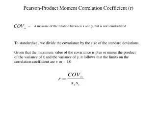
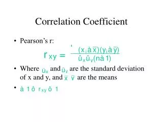
The regression coefficient is an asymmetrical statistic, one that gives different values for the model Y = f(X) and the model X = f(Y). The other major measure of bivariate association is the Pearson product-moment correlation coefficient (sometimes called "little r" for short). The correlation coefficient is a symmetrical statistic. That is, it simply describes the association between X and Y without worrying about whether Y = f(X) or X = f(Y). It would produce the same result in either case. Unlike the regression coefficient, whose values range from 0.0 to , the correlation coefficient ranges from 0.0 when there is NO association between X and Y to 1.00 when there is PERFECT association (either direct or inverse).
To generate the second set of statistics describing association from the linear model, we partition the sum of squares. Graphically, we begin with a single data point, i, in two-dimensional space. Yi is its location on the scale of y (on the y-axis); below that is the predicted location of Y, Yi-hat. The dotted horizontal line (- - - -) is the location of the mean of Y. (When there is no association between X and Y, b = 0.0 and therefore a = Y-bar.) where b = 0,
i Yi• } Yi - hat _ }Y- - - - - - - - - - - - - - - Xi
The vertical line represents the deviation of the ith observation from the mean of Y (i.e., the difference between Yi and Y-bar). The line of best fit bisects the deviation into its two mathematical components. The component ABOVE the line of best fit is the residual, the difference between Yi and Yi - hat, the actual location of the ith observation on the y-axis and the predicted location of this observation on the y-axis. This is the error (or residual) component.
The component BELOW the line of best fit is new. It is the difference between the predicted Y-value, Yi - hat, and the mean of Y (Y-bar). This component is called the regression component. Since these two components combined are the parts of the deviation of the ith observation from the mean of Y, the following is merely an algebraic summary of this relationship:deviation = regression component + error (residual)
Squaring both sides and summing across all observations yieldsorSSTotal = SSRegression + SSError
We can express the amount of association between X and Y as a ratio of the variance explained by the linear model to the total variance in Y to be explained. SSTotal is the variance to be explained and SSRegression the variance accounted for by Y's relationship with X:R2YX = SSRegression / SSTotalThis is the Coefficient of Determination. Its values range from 0.0 when X and Y are independent (i.e., when Y-hat minus Y-bar = 0.0) to 1.0 with perfect association (i.e., SSRegression = SSTotal). It is interpreted as the percentage of the total variance in Y explained by Y's association with X.
In algebraic form, the Coefficient of Determination is calculated asThe denominator is the product of the variance (standard deviation squared) of X and the variance of Y. The numerator is the square of the covariance and can be obtained by squaring the value from the following short-cut equation
In the time and temperature example, N = 3, the sum of X (time) was 23.5, the sum ofthe squared time values was 194.25, the sum of time values squared was 552.25, the sum of Y (temperature) was 248, and the sum of the cross-products was 1,911. sXY = (3)(1911) - (248)(23.5) / (3)(3 - 1)sXY = (5733 - 5828) / 6sXY = - 95 / 6sXY = - 15.833Squaring to get the covariance squared,s2XY = 250.694
Next, we can use the short-hand equation to calculate the two variances:s2X = NX2 - (X)2 / N(N - 1)(Here, the absence of an index and counter on the summation sign implies summing from the first to the last value.)s2X = (3)(194.25) - (23.5)2/ (3)(3- 1)s2X = (582.75) - (552.25) / (3)(2)s2X = 30.5 / 6s2X = 5.083
And for the variance of Y:s2Y = NY2 - (Y)2 / N(N - 1)s2Y = (3)(20,600) - (248)2 / (3)(3 - 1)s2Y = (61,800) - (61,504) / 6s2Y = 296 / 6s2Y = 49.333
Now we can solve for the Coefficient of Determination:R2YX = s2XY / s2X s2YR2YX = 250.694 / (5.083)(49.333)R2YX = 250.694 / 250.760R2YX = 0.9997This is interpreted as meaning that 99.9 percent of the variance in afternoon high temperature is statistically explained by the association of this variable with the time of the sun's first appearance. This is an extremely high—and extremely unlikely—value, since R2YX varies from a minimum of 0.0 (no variance explained) to a maximum of 1.0 (100 percent if ALL the variance is explained).
If the Coefficient of Determination is the percentage of the variance in Y explained by its association with X, then the converse is the percentage of variance in Y NOT explained by its association with X. This is called the Coefficient of Nondetermination, simplyKYX = 1 - R2YXIn this example, the percentage of variance NOT explained is 1 - 0.999, or less than 0.1 percent.
Conceptually, the Pearson product-moment correlation coefficient is the square root of the Coefficient of Determination:For raw data, the correlation coefficient is found byrXY = sXY / sX sYwhere the numerator is the covariance and the denominator is the product of the standard deviations of X and Y. In our example,rXY = - 15.833 / (2.255) (7.024)rXY = - 15.833 / 15.839rXY = - 0.9996
Notice that, unlike the Coefficient of Determination which only takes positive values, the correlation coefficient varies between 0.0 and 1.00. Here, a correlation of - 0.9996 shows an extremely STRONG INVERSE relationship.Finally, in the bivariate situation, the regression coefficient (i.e., slope, b) and the correlation coefficient (rXY) are related, as follows:b = rXY (sY / sX)andrXY = b (sX / sY)
In the present little example,b = (- 0.968) (7.024 / 2.255)b = (- 0.968) (3.115)b = - 3.015andrXY = - 3.115 (2.255 / 7.024)rXY = - 3.115 (0.321)rXY = - 0.999
SAS Time and Temperature ExampleLIBNAME perm 'a:\';LIBNAME library 'a:\';OPTIONS NODATE NONUMBER PS=66;PROC CORR DATA=perm.weather NOSIMPLE;VARtemptime;TITLE1 'Time and Temperature Example';RUN;
Time and Temperature Example Correlation Analysis 2 'VAR' Variables: TIME TEMPPearson Correlation Coefficients / Prob > |R| under Ho: Rho=0 / N = 3 TIME TEMP TIME 1.00000 -0.999830.00.0116 TEMP -0.99983 1.000000.01160.0
Time and Temperature Example Correlation Analysis 2 'VAR' Variables: TIME TEMPPearson Correlation Coefficients / Prob > |R| under Ho: Rho=0 / Number of Observations TIME TEMP TIME 1.00000 -0.999830.00.011623 TEMP -0.99983 1.000000.01160.032
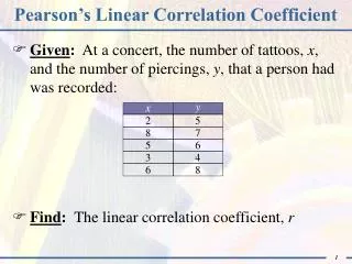
Correlation ExampleFor the following data on ten families, answer the questions below.—————————————————————————————————————————————————————————————————————————————— Annual Income _ Number of _ _ _ Family (in $1,000) (Xi - X)2 Children (Yi - Y)2 (Xi - X)(Yi - Y) X Y—————————————————————————————————————————————————————————————————————————————— 1 25 0 2 17 0 3 20 1 4 14 2 5 11 2 6 10 3 7 6 4 8 8 5 9 8 610 4 7 --- ---X = Y = _ _ X = Y =—————————————————————————————————————————————————————————————————————————————— 1. What is the value of the correlation coefficient? ______________2. What is the value of the Coefficient of Determination? ______________3. What is the value of the Coefficient of Nondetermination? ______________
Correlation Example AnswersFor the following data on ten families, answer the questions below.—————————————————————————————————————————————————————————————————————————————— Annual Income _ Number of _ _ _ Family (in $1,000) (Xi - X)2 Children (Yi - Y)2 (Xi - X)(Yi - Y) X Y——————————————————————————————————————————————————————————————————————————————1 25 161.29 0 9 -38.1 2 17 22.09 0 9 -14.1 3 20 59.29 1 4 -15.4 4 14 2.89 2 1 -1.7 5 11 1.69 2 1 1.3 6 10 5.29 3 0 0.0 7 6 39.69 4 1 -6.3 8 8 18.49 5 4 -8.6 9 8 18.49 6 9 -12.910 4 68.89 7 16 -33.2 --- ---X = 123 Y = 30 _ _ X = 12.3 Y = 3.0 = 398.1 = 54 = -129—————————————————————————————————————————————————————————————————————————————— 1. What is the value of the correlation coefficient? -0.8802. What is the value of the Coefficient of Determination? 0.7743. What is the value of the Coefficient of Nondetermination? 0.226