Download
1 / 36
360 likes | 474 Vues
This presentation explores emerging methodologies in buried object identification, consisting of two parts. The first part focuses on the physics-derived basis for pursuing buried object identification, presenting the electromagnetic induction principles used in metal detectors and their interaction with buried objects. The second part introduces a fast 3D blind deconvolution technique to enhance detection performance. Through various models and simulations, the discussion covers secondary magnetic fields, object polarizability, and their effects on detection accuracy.

E N D
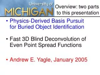
Overview: two parts to this presentation • Physics-Derived Basis Pursuitfor Buried Object Identification • Fast 3D Blind Deconvolution of Even Point Spread Functions • Andrew E. Yagle, January 2005
Metal Detector Coil Voltage Response Buried Object Part I of this Presentation Springfield, VA, January 2005 Physics Derived Basis Pursuit in Buried Object Identification Jay A. Marble and Andrew E. Yagle
Secondary Magnetic Field P r i m a r y M a g n e t i c F i e l d A i r G r o u n d Induced Sources Source Air Horizontal Dipole Vertical Dipole Ground Metal Detector Phenomenology • An Electromagnetic Induction (EMI) Metal Detector utilizes • a coil of wire to generate a magnetic field. • This magnetic field interacts with a buried object inducing “swirling” • electrical (eddy) currents. These induced currents form secondary • sources, which can be modeled as vertical and horizontal dipoles. • The metal detector coil is then switched from a transmitter to a receiver. Coil + - Buried Object Response Transmitted Fields Fields at Buried Object Induced Sources (approximation)
Secondary Magnetic Field Source Air P r i m a r y M a g n e t i c F i e l d A i r G r o u n d Buried Sphere Ground EMI Phenomenology Simplified EMI System Concept Current Source Data Storage Electronics & Sampler Source H-field Metal Object Reaction Incident Field at Object
Source Air Ground EMI Phenomenology (x,y,h) (x,y,-d) Source H-field
Secondary Magnetic Field pz pr EMI Phenomenology * Model assumes a solid spherical target. Metal Object Reaction
Induced Magnetic Sources pz px EMI Phenomenology * Model no longer assumes a solid spherical target. Target Magnetic Polarizability Vector H0x – Horizontal magnetic field at the center of the target produced by the source magnetic dipole. Hxz – Vertical magnetic field at the receive coil produced by the horizontal induced magnetic dipole. H0z – Vertical magnetic field at the center of the target produced by the source magnetic dipole. Hzz – Vertical magnetic field at the receive coil produced by the vertical induced magnetic dipole.
Horizontal Dipole Vertical Dipole Physics Derived Basis Functions • The horizontal dipole produces • the W basis. • The vertical dipole produces • the L basis. TheW Basis Function The L Basis Function
Physics Derived Basis Functions • The spatial signal is • composed of the L(x) • and W(x) basis functions. • The basis functions are • parameterized by depth. • Any object at the same depth • will have the same basis. • The object’s shape affects the • weighting coeffs “a” and “b”. d – depth of buried object a – Polarizability of object in Z-direction. b – Polarizability of object in X-direction.
Canonical Depths • These 3 signals come from identical spheres at different depths. Sphere at 0.0m Sphere at 0.25m Sphere at 1.0m All objects simulated at 0.25m depth.
aL Component aL Component aL Component bW Component bW Component bW Component Canonical Depths • These 3 signals come from identical spheres at different depths. Sphere at 0.0m Sphere at 0.25m Sphere at 1.0m
Wd 62° Ld 2D Signal Subspace Higher Dimensional Space Wd • The natural Ld and Wd • bases are non-orthogonal. • An interesting fact is that • the Ld and Wd bases form • an angle of 62° regardless • of object depth d. • All metal objects at this depth • will exist in this signal • subspace. Ld 2D Plane Spanned by Ld and Wd
Subspaces for Objects at Different Depths Second Depth Subspace Wd2 Wd1 Ld2 Ld1 First Depth Subspace • The bases of objects at a • second depth, Ld2 and Wd2, • span a second plane that • is non-orthogonal to • the plane spanned by the • first depth bases, Ld1 and Wd1.
Canonical Shapes • All 3 of these signals are represented by a vector in the same 2D subspace. Sphere Cylinder Flat Plate All objects simulated at 0.25m depth.
Canonical Shapes • All 3 of these signals are represented by a vector in the same 2D subspace. Sphere Cylinder Flat Plate aL Component aL Component aL Component bW Component bW Component bW Component All objects simulated at 0.25m depth.
Effect of Object Shape, Size, and Content 2D Subspace for Objects at Depth “d” Wd • The object’s polarizability • (the a and b coeffs) • determines the angle • of the signal in the 2D • subspace. • Increasing the object’s • size increases the • weightings, a and b. • More conductive metal • also increases the • weightings, a and b. Larger or More Conductive Sphere Larger or More Conductive Cylinder 45°-Sphere 30°-Cylinder Larger or More Conductive Flat Plate 62° 10°-Flat Plate Ld
Subspace Identification Using Projections
Subspace Identification Performance Deep Sphere Mid Depth Sphere Deep Sphere Mid Depth Sphere Deep Sphere Mid Depth Sphere
New EMI Modality Georgia Tech EMI 600Hz to 60kHz
Part II of this Presentation Fast 3D Blind Deconvolution of Even Point Spread Functions Andrew Yagle and Siddharth ShahThe University of Michigan, Ann Arbor
Motivation Many blind deconvolutionalgorithms need an initial PSF estimate Can be tedious and problematic to measure PSF accurately Blind Deconvolution (Don’t need PSF) BUT But Blind Deconvolution algorithms tend to be slow !Also many still need initial PSF estimate What we need A fast algorithm that performs blind deconvolution
We will show: • An algorithm that performs blind deconvolution that is • Fast • Parallelizable • A linear algebraic formulation • Non iterative (at least for the Least Squares solution)
Assumptions Reasonable in optics. PSFs are symmetric in x, y, and z. Hence h(x,y,z) = h(-x,-y,-z) 1. Point Spread Function or PSF h(x,y,z) is even in 3-D. 2. We know the PSF or image support size. 3. Image has compact support. Potential Problem: Asymmetric PSFs due to optical aberrations Can these be solved too ? YES (later)
Formulation DATA PSF OBJECT NOISE y(i1,i2,i3) = h(i1,i2,i3) *** u(i1,i2,i3) + n(i1,i2,i3) whereu(i1,i2,i3) ≠ 0 for 0 ≤ i1,i2,i3 ≤ M-1 h(i1,i2,i3) ≠ 0 for 0 ≤ i1,i2,i3 ≤ L-1 y(i1,i2,i3) ≠ 0 for 0 ≤ i1,i2,i3 ≤ N-1 N=L+M-1 h(i1,i2,i3) = h(L-i1,L-i2,L-i3) (even PSF)n(i1,i2,i3) is zero mean white Gaussian noise. Given only datay(i1,i2,i3) reconstruct the object u(i1,i2,i3)and the PSF h(i1,i2,i3) PROBLEM
1-D Solution Equating coefficients, we get the following matrix Toeplitz Structure
2-D Problem or Example Solve:
2-D Example Solution Size of matrix (2M + L- 2)2 X (2M2) Toeplitz Block Toeplitz structure
3-D Solution Equating coefficients we would get a doubly nested Toeplitz matrix Matrix size: (2M + L-2)3 X (2M)3 Q: So we have solved the 3D problem ? A: Not quite !! If M=5 and L=3 then the matrix size is 4913 X1024 It will be intractable to use this method “as is” in 3D !
FourierDecomposition 0 ≤ k ≤ M-1 Using conjugate symmetry The point ? The last equation is decoupled into a set of M 2D problems !
2-D to 1-D So we broke down a huge 3D problem to M simpler 2D problems What next ? Substitute for xk in each 2D problem and you would get M 1D problems in z To summarize We broke up a large 3D problem into M2 1D problems
2-D scale factors Note that each 1D problem will be correct upto a scale factor. Each row is solved to a scaled factor. Decoupling 2D to 1D How do we get the whole 2D solution correctly ? Solve along columns and compare coefficients 1D FT along columns solve d1U(:,1) d4U(:,4) d2U(:,2) d3U(:,3) 1D FTalong rows c1U(1,:) c2U(2,:) U(x,y) solve c3U(3,:) c4U(4,:) Compare and scale
3-D scale factors We just learned how a 2D problem could be correctly scaled Solve 3D Decouple 3D to 2D Decouple 2D to 1D Solve 1D Scale 2D Solns 2D solutions Scale 1D Solns Solve 2D problems d2 d1 Decouple along x U(x,y,z) Decouple along z Compare and scale 2D problems c1 c2 Solve 2D problems
Stochastic Case In presence of noise the nullspace of the toeplitz structure no longer exists. We can find “nearest” nullspace using Least Squares (LS) (fast) Can use structure of matrix to solve by structured least squares (STLS)(slow but more accurate) We can show that such norm minimization will give us the Maximum Likelihood Estimate of the object u(x,y,z)
Simulations Synthetic bead image (30X30X30), (3X3X3) PSF, no noise
Stochastic case: STLN vs. LS Least Squares v/s STLN comparison 7X7X7 image. 3X3X3 PSF. 50 iterations per SNR Least squares does well at high SNRs but at low and medium SNRS STLN is better.
SNR SNR Comparison with Lucy Richardson Time MSE Our algorithm need only a fixed amount of time to solve independent of the SNR. LR needs more time and time to solve depends on the SNR. Our algorithm gave a lower MSE. In LR Final accuracy even in absence of noise depends on initial PSF estimate.