Preliminary LES simulations with Méso-NH to investigate water vapor variability during IHOP_2002

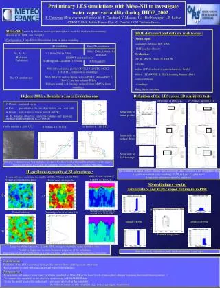
1. Visible satellite at 2000 UTC  Profiles at 1130 UTC rv Profiles at 1130 UTC Preliminary LES simulations with Méso-NH to investigate water vapor variability during IHOP_2002 F. Couvreux (fleur.couvreux@meteo.fr), F. Guichard, V. Masson, J.-L. Redelsperger, J.-P. Lafore CNRM-GAME, Météo-France,42,av. G. Coriolis 31057 ToulouseFrance Méso-NH: a non-hydrostatic mesoscale atmospheric model of the french community (Lafore et al., 1998, Ann. Geoph.) Configuration: Large Eddies Simulation from an initial sounding • IHOP data used and data we wish to use : • Model input: • soundings (Mobile, ISS, NWS) • - ISSF (surface fluxes) • Evaluation: • AERI, MAPR, HARLIE, FMCW • satellite • radars (S-Pol: reflectivity and refractivity fields) • lidars (LEANDRE II, DIAL,Scaning Raman Lidar) • surface stations • soundings • King-Air in-situ data 1D simulation First 3D simulation 100m, 100m, 100m to be increased \, \, from 20m to 250m x, y, z Radiation Turbulence ECMWF radiation code 1D (Bougeault-Lacarrere) 1.5 order 3D (Deardoff) With different initial profiles (MGL2-1120UTC, MGL2-1216UTC, composite of soundings) The 1D simulations : With different surface fluxes (station ISSF 1, station ISFF 2, Bo=1/2, surface scheme ISBA) Without or with L-S forcings deduced from MM5 or from soundings 14 June 2002, a Boundary Layer Evolution case Definition of the LES: some 1D sensitivity tests  Profiles at 1800 UTC rv Profiles at 1800 UTC DDC • Clouds : scattered cirrus • Past : precipitation the two days before => wet soils • Winds : light winds (< 6m/s) from N and NE • BL structure observed: convective plumes and growing thermals in the afternoon, hCBL1500 m ISSF-3 MGL2_1216 MGL2_1120 Composite_1130 I.P.=MGL2-1120 I.P.=MGL2-1216 I.P.=composite I.P.=MGL2-1120 I.P.=MGL2-1216 I.P.=composite Sensitivity to initial profile ISSF-2 SPol MGL1-others ISS MCLASS-11h MGL2-11-13 ISSF-1 MGL1-11h MGL2-14h.. VICI AMA Fx=Bo=2/3 Fx=Bo=1/2 Fx=isba Fx=ISSF2 Fx=ISSF1 Fx=Bo=2/3 Fx=Bo=1/2 Fx=isba Fx=ISSF2 Fx=ISSF1 Sensitivity to surface fluxes N S N S Sensitivity to L-S forcings Forc=adv h. MM5 Forc=adv h. soundings Forc=None Forc=adv h. +w MM5 Forc=adv h. MM5 Forc=adv h. soundings Forc=None Forc=adv h. +w MM5 This day is characterized by a high pressure and a North(-)-South(+) humidity gradient over the region. Several dry layers are visible on soundings (for example VICI) - complexe structures. 3D-preliminary results of BL structures : The definition of initial profiles, surface fluxes and large-scale advection is not straightforward. A significative small-scale variability (1-2 K in  and 1-2 g/kg in rv). Large-scale advection cannot be neglected. Horizontal cross section in the middle of CBL (700 m) at 2100 UTC Vertical cross section of  and w at 2100 UTC Virtual potential temperature Water vapor mixing ratio 3D-preliminary results: Temperature and Water vapor mixing ratio PDF v rv Mixing ratio Vertical cross section of rv and w at 2100 UTC Vertical velocity Vertical profile of w² after 21h altitude =800m altitude =1500m w Potential temperature Large variability (v, rv, w…) in the CBL, strongest variability in the inversion zone. Available diagnostics to study statistical properties of the turbulence. Importance of the role of thermals as a source of water vapor and potential temperature variability. Statistical tools available to study the distribution of water vapor • Conclusions : • Definition of the LES case study (initial profile, surface fluxes and large-scale advection). • Tools available to study turbulence and water vapor heterogeneities. • Perspectives : • To determine and analyze water vapor variability simulated by Méso-NH in the lower levels of atmosphere (diurnal variations, horizontal heterogeneities...) • To compare this variability to the observed one focusing on LEANDRE II data • To use the model as a tool to understand : - processes involved in this variability • - the different sources of this variability (e.g., using Lagrangian trajectories)