The Binomial Model

1. The Binomial Model $120 $20 $100 C100 = ? $90 $0 Strategy: Buy 1 stock sell 1.5 calls

2. The Binomial Model CF today CF at T (S = 90) CF at T (S=120) Buy Stock -$100 $90 $120 Sell 1.5 calls $1.5C $0 -$30 ____________ _________ _______ 1.5C - 100 $90 $90

3. The Binomial Model • Investment today of $100-1.5 C yields $90 for sure. Hence, • [100-1.5C](1+r) = 90 • If r=10% • C = (1/1.5)[100-90/1.1] = 12.12

4. The Binomial Model $uS Cu $S 1/Δ – hedge ratio $C $dS Cd uS - (1/Δ)*Cu S – (1/Δ)*C dS - (1/Δ)*Cd

5. Delta • Chose 1/Δ to hedge, thus; uS - (1/Δ)*Cu = dS - (1/Δ)*Cd 1/Δ = {uS – dS}/{Cu – Cd}

6. Delta $120 $20 = 0 - $0 $90

7. The Binomial Model uS – {1/Δ}*Cu S – {1/Δ}*C Investment Certain outcome {S – [1/Δ}*C}*R = uS – {1/Δ}*Cu R = 1 + rf and u > R > d C = {S(R-u) + (1/Δ)Cu}/(1/Δ)R

8. The Binomial Model • Substitute for 1/Δ to get • C = {P*Cu + (1-P)*Cd}/R • P = [R-d]/[u-d]

9. The Binomial Model • In our example: u=1.2, d=0.9, R=1.1, uS=120, ds=90, E = 100, S=100 • P =[R-d]/[u-d] = [1.1-0.9]/[1.2-0.9]=2/3 • C= {(2/3)*20 + (1/3)*0}/1.1 = 12.12

10. What is P? u > R > d 0 < P < 1 R=1.1 ________________________________ d=0.9 u=1.2

11. What is P? • P cannot be a probability since we do not know the probability of a price increase – denoted q. • Since the valuation of C is true for any q we can assume (for our example) q = 0.5 • Do you feel comfortable with q = 0.5?

12. What is P? • But if q=0.5 we can compute the expected return of the stock. • E(Rs) = 0.5*20% + 0.5*(10%) = 5% • Hence, E(Rs) < rf

13. What is P? • Assume q=7/8=0.875. • In our example P=[1.1-0.9]/[1.2-0.9] = 2/3 • E(Rs) = 0.875*20% + 0.125*(10%) = 16.25% • Risk premium = 16.25 – 10 = 6.25%

14. What is P? • Now reduce the risk aversion in the economy by reducing the risk premium to 1.25%. Increase the risk free rate to 15%. • P = [1.15-0.9]/[1.2-0.9] = 5/6 = 0.833 • P gets closer to q • C=5/6*20/1.15 = 14.493

15. What is P? • Pushing it one step further, lets reduce the risk aversion in the economy to zero – R=1.1625 • P = [1.1625-0.9]/[1.2-0.9] = 7/8 • P is now equal to q • C = {7/8}*20/1.1625 = 15.054

16. P – the risk neutral probability P < q Risk Aversion P = q Risk neutral P > q Risk seeking

17. P – the risk neutral probability $20 $20 0.875 0.666 0.333 0.125 $0 $0 0.875*20=17.5 0.666*20=13.333 17.5/1.1=15.909 13.333/1.1=12.12

18. Certainty equivalent • The difference 17.5 – 13.333 = 4.167 is a correction for risk in the numerator • The option model is valuation by certainty equivalents. • Once we use P as if it is q we can take expectations and discount with the risk free rate

19. Two periods {0.666*44+0.333*8}/1.1 144 44 120 29.09 108 100 19.08 8 90 4.844 81 0 {0.666*29.09+0.333*4.844}/1.1 {0.666*8/1.1

20. Two Periods • Cu = {P*Cuu + (1-P)*Cud}/R • Cd = {P*Cud + (1-P)*Cdd}/R • C = {P*Cu + (1-P)*Cd}/R • C = {P2 Cuu + 2P(1-P)Cud + (1-P)2 Cdd}/R2

21. Four periods 1 u4 P4 4 du3 P3 (1-P) 6 1 d2u2 P2(1-P)2 4 d3u (1-P)3 P 1 d4 (1-P)4

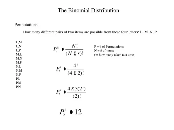
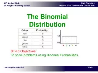
22. The Binomial Distribution • The probability of a path with j ups and n-j downs is Pj(1 – P)n-j • The number of paths leading to a node is n!/{j!(n-j)!} • The probability to get to a node is {n!/j!(n-j)!}Pj(1-P)n-j

23. The Binomial Distribution • The probability to get to any one of the nodes is Σj=0 [{n!/j!(n-j)!}Pj(1-P)n-j] = 1 • The probability of at least a ups is Φ{a, n, P} = Σj=a{[n!/(j!(n-j)!]Pj(1-P)n-j} < 1

24. The Binomial Option Pricing Model C = [Σj=0{n!/j!(n-j)!}Pj(1-P)n-jMax{0, ujdn-jS – E}]/Rn Let a (number of ups) be the smallest integer such that the option will mature in the money

25. The Binomial Option Pricing Model C = [Σj=a{n!/j!(n-j)!} Pj(1-P)n-j {ujdn-jS – E}]/Rn = S[Σj=a{n!/j!(n-j)!} Pj(1-P)n-j{ujdn-j/Rn} - ER-n[Σj=a{n!/j!(n-j)!} Pj(1-P)n-j]

26. The Binomial Option Pricing Model S[Σj=a{n!/j!(n-j)!} [u/R]jPj (1-P)n-j {d/R}n-j } Let P’ = [u/R]P than 1 – P’ = [u/R]{(R-d)/(u-d)} = [d/R](1-P) S[Σj=a{n!/j!(n-j)!} P’j (1-P’)n-j]

27. The Binomial Option Pricing Model • C = S*Φ{a, n, P’} - E*R-n*Φ*{a, n, P} • Σj=0{[n!/(j!(n-j)!]Pj(1-P)n-j}= 1 • Φ{a, n, P} = Σj=a{[n!/(j!(n-j)!]Pj(1-P)n-j} < 1

28. The Binomial Option Pricing Model • C = S*Φ{a, n, P’} - E*R-n*Φ*{a, n, P} • P = [R-d]/[u-d] • P’ = [u/R]P