Download
1 / 11
110 likes | 198 Vues
Discover the benefits of fluxons in MHD codes, their unique features, and future applications. Learn how fluxons are reshaping magnetic field modeling and the key advancements made by the SwRI fluxon code. Understand the challenges of existing MHD codes and how fluxons offer a promising solution.

E N D
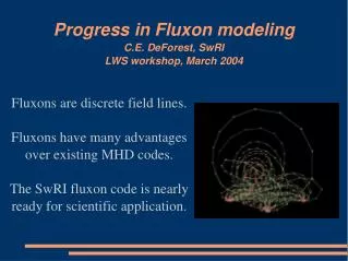
Fluxons are discrete field lines. Fluxons have many advantages over existing MHD codes. The SwRI fluxon code is nearly ready for scientific application. Progress in Fluxon modelingC.E. DeForest, SwRILWS workshop, March 2004
Gripes about existing MHD codes... • Eulerian grids are too resistive. • Lagrangian grids fail in evolving systems. • 3-D models choke even huge computers.
What are fluxons, and what makes them so great? • Fluxons are quantized field lines that interact at a distance. • They are modeled as lists of nodes located in 3-space. • Forces are calculated via analytic geometry. • Current code: finds force-free fields by magnetofriction. • Future code: quasi-stationary MHD, then full MHD. • Fluxon models are divergence-free by construction. • Boundaries: none (no box!) • Reconnection: none unless you add it, which is easily done. • Node count scales as O(L2.1)-O(L2.4) for 3-D simulation.
Adapting Maxwell's Equations to Fluxons... Magnetic energy in a volume: Force resolves to the magnetic pressure and curvature forces: How to estimate B from the geometry?
Voronoi Analysis: 3-D The B field is just each fluxon's flux, divided by the cross-section of its neighborhood and directed along the fluxon. Voronoi mathematics deals with related problems. Finding the 3-D neighborhood is tractable but expensive.
Voronoi Analysis: 2-D (Cross-sectional Plane) Working in the cross-sectional plane makes finding the Voronoi neighborhood affordable. The geometry of the neighborhood gives both the magnetic pressure and its gradient.
Simple 3-D Relaxations Fluxon relaxation in simple cases yields familiar answers. Potential field animation Simple current animation
Interacting flux A low (freshly emerged?) potential field bipole interacts with a simple current-carrying loop.
Performance, and future milestones: • Those relaxations used 20 - 45 min. on a 1GHz Pentium laptop; 500-1,000 nodes each. • Not optimized for speed. 10x-30x speedup feasible. • 104-105 nodes: OK for workstation. ('toy' problems) • 106-107 nodes: OK for big iron. (AR or global models) • Validate code; write easier front-end. • Augment to track tension build-up as boundary evolves. • Add reconnection criteria. • Add non-magnetic forces. • Add inertial forces.
Some applications (Tomorrow, the world!)... • Effect of magnetic carpet on corona • Heating and evolution of active regions • Aly-Sturrock conjecture (in-)validation • CME onset; filament stability, formation, & support • Interaction of plasmoids with the magnetosphere • Real-time CME prediction (using HVMI & AIA)