
Finding Boundaries
E N D
Presentation Transcript
09/28/11 Finding Boundaries Computer Vision CS 143, Brown James Hays Many slides from Lana Lazebnik, Steve Seitz, David Forsyth, David Lowe, Fei-Fei Li, and Derek Hoiem
Edge detection • Goal: Identify sudden changes (discontinuities) in an image • Intuitively, most semantic and shape information from the image can be encoded in the edges • More compact than pixels • Ideal: artist’s line drawing (but artist is also using object-level knowledge) Source: D. Lowe
Why do we care about edges? Vertical vanishing point (at infinity) Vanishing line Vanishing point Vanishing point • Extract information, recognize objects • Recover geometry and viewpoint
Origin of Edges • Edges are caused by a variety of factors surface normal discontinuity depth discontinuity surface color discontinuity illumination discontinuity Source: Steve Seitz
Closeup of edges Source: D. Hoiem
Closeup of edges Source: D. Hoiem
Closeup of edges Source: D. Hoiem
Closeup of edges Source: D. Hoiem
Characterizing edges intensity function(along horizontal scanline) first derivative edges correspond toextrema of derivative • An edge is a place of rapid change in the image intensity function image
Intensity profile Source: D. Hoiem
With a little Gaussian noise Gradient Source: D. Hoiem
Effects of noise Where is the edge? • Consider a single row or column of the image • Plotting intensity as a function of position gives a signal Source: S. Seitz
Effects of noise • Difference filters respond strongly to noise • Image noise results in pixels that look very different from their neighbors • Generally, the larger the noise the stronger the response • What can we do about it? Source: D. Forsyth
Solution: smooth first g f * g • To find edges, look for peaks in f Source: S. Seitz
Derivative theorem of convolution f • Differentiation is convolution, and convolution is associative: • This saves us one operation: Source: S. Seitz
Derivative of Gaussian filter * [1 -1] =
Tradeoff between smoothing and localization • Smoothed derivative removes noise, but blurs edge. Also finds edges at different “scales”. 1 pixel 3 pixels 7 pixels Source: D. Forsyth
Designing an edge detector • Criteria for a good edge detector: • Good detection: the optimal detector should find all real edges, ignoring noise or other artifacts • Good localization • the edges detected must be as close as possible to the true edges • the detector must return one point only for each true edge point • Cues of edge detection • Differences in color, intensity, or texture across the boundary • Continuity and closure • High-level knowledge Source: L. Fei-Fei
Canny edge detector • This is probably the most widely used edge detector in computer vision • Theoretical model: step-edges corrupted by additive Gaussian noise • Canny has shown that the first derivative of the Gaussian closely approximates the operator that optimizes the product of signal-to-noise ratio and localization J. Canny, A Computational Approach To Edge Detection, IEEE Trans. Pattern Analysis and Machine Intelligence, 8:679-714, 1986. Source: L. Fei-Fei
Example original image (Lena)
Derivative of Gaussian filter y-direction x-direction
Compute Gradients (DoG) X-Derivative of Gaussian Y-Derivative of Gaussian Gradient Magnitude
Get Orientation at Each Pixel • Threshold at minimum level • Get orientation theta = atan2(gy, gx)
Non-maximum suppression for each orientation At q, we have a maximum if the value is larger than those at both p and at r. Interpolate to get these values. Source: D. Forsyth
Hysteresis thresholding • Threshold at low/high levels to get weak/strong edge pixels • Do connected components, starting from strong edge pixels
Hysteresis thresholding • Check that maximum value of gradient value is sufficiently large • drop-outs? use hysteresis • use a high threshold to start edge curves and a low threshold to continue them. Source: S. Seitz
Canny edge detector • Filter image with x, y derivatives of Gaussian • Find magnitude and orientation of gradient • Non-maximum suppression: • Thin multi-pixel wide “ridges” down to single pixel width • Thresholding and linking (hysteresis): • Define two thresholds: low and high • Use the high threshold to start edge curves and the low threshold to continue them • MATLAB: edge(image, ‘canny’) Source: D. Lowe, L. Fei-Fei
Effect of (Gaussian kernel spread/size) original Canny with Canny with • The choice of depends on desired behavior • large detects large scale edges • small detects fine features Source: S. Seitz
Learning to detect boundaries • Berkeley segmentation database:http://www.eecs.berkeley.edu/Research/Projects/CS/vision/grouping/segbench/ human segmentation image gradient magnitude
Representing Texture Source: Forsyth
Texture and Material http://www-cvr.ai.uiuc.edu/ponce_grp/data/texture_database/samples/
Texture and Orientation http://www-cvr.ai.uiuc.edu/ponce_grp/data/texture_database/samples/
Texture and Scale http://www-cvr.ai.uiuc.edu/ponce_grp/data/texture_database/samples/
What is texture? Regular or stochastic patterns caused by bumps, grooves, and/or markings
How can we represent texture? • Compute responses of blobs and edges at various orientations and scales
Overcomplete representation: filter banks LM Filter Bank Code for filter banks: www.robots.ox.ac.uk/~vgg/research/texclass/filters.html
Filter banks • Process image with each filter and keep responses (or squared/abs responses)
How can we represent texture? • Measure responses of blobs and edges at various orientations and scales • Idea 1: Record simple statistics (e.g., mean, std.) of absolute filter responses
Can you match the texture to the response? Filters A B 1 2 C 3 Mean abs responses
Representing texture • Idea 2: take vectors of filter responses at each pixel and cluster them, then take histograms.
Building Visual Dictionaries • Sample patches from a database • E.g., 128 dimensional SIFT vectors • Cluster the patches • Cluster centers are the dictionary • Assign a codeword (number) to each new patch, according to the nearest cluster
pB boundary detector Martin, Fowlkes, Malik 2004: Learning to Detect Natural Boundaries… http://www.eecs.berkeley.edu/Research/Projects/CS/vision/grouping/papers/mfm-pami-boundary.pdf Figure from Fowlkes
pB Boundary Detector Figure from Fowlkes
Brightness Color Texture Combined Human
Global pB boundary detector Figure from Fowlkes
45 years of boundary detection Source: Arbelaez, Maire, Fowlkes, and Malik. TPAMI 2011 (pdf)