Download
1 / 36
540 likes | 976 Vues
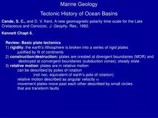
Marine Geology Tectonic History of Ocean Basins Cande, S. C., and D. V. Kent, A new geomagnetic polarity time scale for the Late Cretaceous and Cenozoic, J. Geophy. Res., 1992. Kennett Chapt 6. Review: Basic tenants of plate tectonics

E N D
Marine Geology • Tectonic History of Ocean Basins • Cande, S. C., and D. V. Kent,A new geomagnetic polarity time scale for the Late Cretaceous and Cenozoic, J. Geophy. Res., 1992. • Kennett Chapt 6. • Review: Basic tenants of plate tectonics • 1) rigidity: the earth's lithosphere is broken into a series of rigid plates • justified by fit of continents • 2) construction/destruction: plates are created at divergent boundaries (MOR) and • destroyed at convergent boundaries (subduction zones); steady state • 3) relative motion: plates are in relative motion • can be described by poles of rotation • (not nec. equivalent of earth's pole of rotation); • relative motion described as angular velocity • movement plates move past each other described by small circles • that are transform faults
Gravity and the geoid • What is the geoid - gravitational equipotential surface = • a ball place on it will not roll. lines of equi-potential must move up over a + anomaly to stay at the same field intensity • Map of geoid, noting the 180 m relief between New Guinea and India • Tectonic features can be mapped with gravity (all of the wonderful maps) • For example: Fracture zones are sources of gravitational disequilibrium • offsets in age (= thermal cooling), offsets in density (transform fault) • offsets in age, elastic response to load (fracture zone) + - couple • What the data look like
Filtered geoid height from Seasat data showing fracture zones use these data to map fracture zones (Cande et al., 1988)
Magnetics • tow a proton precession magnetometer behind ship ("maggie") or • from airplane (aeromag data)what do you expect for a magnetic anomaly? deviations (in gammas) from expected magnetic field; remove effects of latitude (reduce to the pole/deskew) • generic anomalies generally due to presence of magnetized crustal rocks • after corrections (reduce to the pole/deskew) • highly magnetized in present direction (normal) yields positive magnetic anomaly • e.g., MMA in South Atlantic (Eltanin)
For example • Marine Magnetic Anomalies (MMA) • in South Atlantic • (Eltanin) • Pitman's discovery on Eltanin 19 profile
mapped on various ridge crest, • e.g., Reykjanes Ridge south of Iceland • Vine-Matthews '63, • Carlsberg Ridge. • "seafloor spreading as a...
Seafloor spreading as a magnetic tape recorder Explains symmetry on ridges of MMA; yields a prediction for ages of MMA What is the spreading rate in the above example? Answer : 400 km/10 m.y. = 40 km/m.y. = 4,000,000 cm/1,000,000 years = 4 cm/year (half rate; ocean basin opens 8 cm/yr)
So. Atlantic • No. Pacific • So. Pacific Heirtzler et al. showed on ridges throughout world
the first geomagnetic polarity time scale: GPTS • radiometric age measurement and • rock magnetics • Cox and Dalrymple (CA, Snake R.); McDougall and Tarling in Hawaii • yields a prediction for ages of MMA
Heirtzler et al (1967) assumed constant seafloor spreading rates in the South Atlantic from 0 Ma to3.4 Ma (interpolation), and then extrapolated this rate back to some 80 Ma!!!!!! today: his guess was accurate within about 10% • Heirtzler et al. (1968; HDHPL68) extended back with a grand extrapolation • based on one profile in S. Atlantic V20, • calibration at 0, 3.4 Ma: 20 fold extrap.!! • prediction of ages with distance tested by Leg 3 • Where do geological boundaries come from • E/O was thought to be ~38 Ma, therefore Heirtzler put it there. • It is a GPTS, but not really a geological time scale
e.g., • Site 14 bottomed in upper • Eocene strata; • time scales said that this must • be about 40Ma • -- showed that the ages • increased monotonically, • symmetrically • on either side of ridge • --"proved seafloor spreading"
Heirtzler et a. (1967) assumed constant spreading rates in the South Atlantic and a typical profile question: how well do we know polarity sequence? it is all relative!@%^$!! every profile suffers from irregularities: asymmetric spreading, ridge jumps, propagating rifts • ...
calculate finite rotation polesnecessary to move matching anomaly pairs and fracture zones together (e.g., Cande et al, 43 poles for the S. Atlantic) • use magnetic anomalies and fracture zone rotated back according to the pole of rotation • project distance between anomalies onto a synthetic flow line • provides: • 1) a new time scale once calibrated • 2) a means of evaluating tectonic changes in great detail
check pole accuracy by plotting virtual fracture z ) calculate stage poles (rotation between individual magnetic anomalies) gives actual motion direction and rate with time
Cande and Kent 1992 - used results of Cande et al '88 to make the ultimate • Magnetic Anomaly compilation and Geomagnetic Polarity Time Scale • generate 9 stage poles from the set of 43 finite poles, (≈ evenly spaced, well-defined, well dated via biostratigraphy and isotope dates) anomalies to define the virtual fracture zone in center of S. Atlantic stage poles (rotation between individual magnetic anomalies) gives actual motion direction and rate () with time • note that for the S. Atlantic there are some significant changesnote that now the pole requires a reference frame (e.g., holding Africa fixed; hot spot; etc.)
... 1) stack de-skewed So. Atlantic magnetic anomaly pattern to define Chrons
2) go to well-studied ridges with multiple magnetic lines to obtain more detailed magnetics • ... • 3) go to faster-spreading ridges (Pacific) to locate "tiny wiggles" <500 k.y. magnetic anomalies
... • Impose 2 and 3 on spacing • defined by #1, the S. Atlantic • Finally, remove tiny wiggles of • < 30 k.y. duration (uncertain or inconsistent); • obtain a polarity vs. distance record
... • Last, impose an age model, assuming no rapid changes in spreading rate (cubic spline fit of ages to anomalies • used to define poles)
CK92: • Late Cretaceous (Campanian; ~83 Ma) to Recent: • Anomalies 33 to 1 (Bruhnes) • Cretaceous quiet zone (A34): long interval of normal polarities and crust (83-120 Ma) • M series ("Keathly") anomalies M0-M25 (120-160 Ma magnetic anomalies on ocean floor (ex. S.Atlantic, Cande) • ...
Implications for spreading rates • S. Atlantic - reduces rapid variations required by earlier magnetic time scale • Central Atlantic - reduces rapid variations required by other magnetic time scales to A22 time (≈ 50 Ma)
North Pacific - increases variations Major global tectonic reorganization C24r (Paleocene/Eocene boundary; opening of Norwegian-Greenland Sea; ~56-53.25 Ma Large global tectonic reorganization M10n (not shown) ~132-130 Ma; early Hauterivian Early Early Cretaceous
Tectonic history oldest definite ocean crust 165 Ma; could be as old as 180 Ma Pangea: all continents assembled together intact only lasted a short time (280-180 Ma); ocean Panthalassa; Tethys: an embayment of Panthallassa Mediterranean is remnant of Tethys
Pacific 3 sets of M-series lineations: (Mesozoic older than quiet zone) Japanese, Hawaiian, Phoenix magnetic
where were the plates? How do they know? use magnetic anomalies to define paleo-pole allows paleoreconstruction Problems quiet zone destroyed plates uncertain plate circuit are hot spots fixed? Plate destruction three destroyed plates: Kula, Farallon, Phoenix • ... What is the mean age of ocean crust??? Pacific Ocean: Pacific, Antarctic, Nazca, Cocos Plates
Global Ocean Floor Age Müller et al.,1997
Subduction of ridge modern Gulf Ca/San Andrea Fault system Juan de Fuca ridge remnant of rapid (>5 cm/yr) subduction of Farralon plate
breakup of Pangea: opening of the Atlantic 1) continental rifting Late Triassic to Early Jurassic (ca. 215-185 Ma) analog to modern African rift valley 2) breakup unconformity 3) 185-165 Ma seafloor spreading in North Atlantic began in Middle Jurassic (Callovian 165 Ma oldest definite) narrow ocean: thick salt deposits Red Sea analog 125-110 Ma: opening of So Atlantic unconnected to North Atlantic opening of Labrador Sea (ca. 75-35 Ma; A32-A13) opening of Norwegian-Greenland Sea A24r time (ca. 55 Ma) no/little opening to Arctic prior Greenland-Scotland Ridge: barrier; subsidence by Oligocene (ca. 35 Ma); history is controversial: some say not till mid-Miocene • ...
125-110 Ma: opening of So Atlantic unconnected to North Atlantic Giant mediterranean sea Subsidence and opening to north by 110 Ma Subsidence of passages to deep-water flow (Rio Grande Rise) by 70 Ma • ...
Indian Ocean most complicated 90-53 Ma: spectacular northern motion of Australia two great transform faults: Chagos-Lacadive (w) and Ninetyeast R. (e) (examine map) India collision Asia, began Eocene 50 Ma, "hard collision" Miocene mountain building resulting of collision of two continents can't subduct cont. crust
... separation of Australia from Antarctica in late K, sped up in early Eocene Opening of Drake Passage in late Eocene to early Miocene
... Last 15-30 m.y. spreading rates, quite variable from ocean to ocean SE Indian Ridge- decreases variations ≈ 10 to 30 k.y., similar for older times