Market Risk VaR: Model-Building Approach
720 likes | 1.04k Vues
Market Risk VaR: Model-Building Approach. The Model-Building Approach. The main alternative to historical simulation is to make assumptions about the probability distributions of the returns on the market variables

Market Risk VaR: Model-Building Approach
E N D
Presentation Transcript
The Model-Building Approach • The main alternative to historical simulation is to make assumptions about the probability distributions of the returns on the market variables • This is known as the model building approach (or sometimes the variance-covariance approach)
Example • You invest $300,000 in gold and a $500,000 in silver. • The daily volatilities of these two assets are 1.8% and 1.2% respectively • The coefficient of correlation between their returns is 0.6. • What is the 10-day 97.5% VaR for the portfolio? • By how much does diversification reduce the VaR?
Example continued • The variance of the portfolio (in thousands of dollars) is 0.0182× 3002 + 0.0122 × 5002 + 2 × 300 × 500 × 0.6 × 0.018 × 0.012 = 104.04 • The standard deviation is 10.2 • Since N(−1.96) = 0.025, the 1-day 97.5% VaR is 10.2 × 1.96 = 19.99 • The 10-day 97.5% VaR is × 19.99 = 63.22 or $63,220
Example Continued • The 10-day 97.5% value at risk for the gold investment is 5, 400 × × 1.96 = $33, 470. • The 10-day 97.5% value at risk for the silver investment is 6,000 × × 1.96 = $37,188. • The diversification benefit is 33,470 + 37,188 − 63,220 = $7, 438
The Linear Model We assume • The daily change in the value of a portfolio is linearly related to the daily returns from market variables • The returns from the market variables are normally distributed
Corresponding Result for Variance of Portfolio Value siis the daily volatility of the ith asset (i.e., SD of daily returns) Pis the SD of the change in the portfolio value per day i=wiP is amount invested in ith asset
VaR with Normally Distributed Market Factors • The general form for calculating parametric VaR is: = Average expected return = Standard deviation T = Holding period Z-Score=probability
But the Distribution of the Daily Return on an Option is not Normal The linear model fails to capture skewness in the probability distribution of the portfolio value.
Option Position Risk Management • Option books bear huge amount of risk with substantial leverage in the position. • It is therefore crucial for option book runners to have an accurate and efficient risk management system and methodology. • If not properly implemented, financial institutions may face similar issues to distressed financial institutions like LTCM, Barings, AIG and many more.
“Greeks” • Option price = f(S, E, T, r, σ) • S= price of the underlying asset • E = exercise price • T= time to expiration • r= annualized risk free rate • = volatility of the return on the stock
“Greeks” Delta: sensitivity of the option price or portfolio value to a small change in the price of the underlying asset, S Gamma: sensitivity of the delta to a small change in the price of the underlying asset, S
“Greeks” continued Rho:sensitivity of the option price change to a small change of r Vega: sensitivity of the option price change to a small change of σ Theta (time decay): sensitivity of the option price change to the passage of time.
Black Scholes and “Greeks” • Black-Scholes Option Pricing Formula: Calls: C= S0N(d1) – Ee-rTN(d2) Puts: P= Ee-rTN(-d2) – S0N(-d1) d1=
Black Scholes Delta • Delta: The sensitivity of option price change to a small stock price change Call: 0 ≤ N(d1) ≤ 1 Put : -1 ≤ N(d1) – 1 ≤ 0 • Delta hedging: • – option + delta_stock× S; • This portfolio is called a Delta neutral portfolio. • Perfect delta hedging: If S changes, we need to rebalance the hedging position continuously.
Delta Hedging Call price Slope=Delta=0.6 100 S0 • S0=$100 C=$10 • Short 100 calls • Buy 100 × Delta = 60 shares • - ∆C = +∆S × Delta • if ∆S = +$1 (from $100 to $101) • The change of call price: $1 × 0.6 × 100 = $60 • The change of stock position: $1 × 60 shares = $60
Dynamic hedging v.s. Static-hedging • As stock price keeps changing, the delta will change. Thus, we need to rebalance the portfolio in order to maintain the delta neutral condition. S $110, Delta 0.65. • We need to add extra 5 shares of stock into the portfolio. It’s called dynamic-hedging. If we just leave it alone, it’s called static-hedging • Problem of Delta-neutral hedging: If Delta is extremely sensitive to stock price changes, we need to rebalance the portfolio continuously.
Black Scholes Gamma Gamma: Sensitivity of the delta change to a small change of S Gamma E S0
Gamma (cont.) • The delta of ATM options has the highest sensitivity to a stock price change. • For ATM options, as time passes away, the gamma increases dramatically, because ATM value is very sensitive to jumps in stock prices. • If Port > 0, the value of the portfolio will increase as S moves (either up or down). • If Port < 0, the value of the portfolio will decrease as S moves (either up or down).
Skewness of the distribution of the return on the option Positive Gamma Negative Gamma
Translation of Asset Price Change to Price Change for Long Call Long Call Asset Price
Translation of Asset Price Change to Price Change for Short Call Asset Price Short Call
Delta-gamma-hedging • To make the delta-neutral portfolio into a Delta-gamma neutral portfolio, we need to: • Add certain amount of other options into the portfolio: NG × G + = 0 (NG= -/ G is number of new options; G is gamma of the new options) 2. Adjust number of stocks to make the new portfolio delta-neutral.
Delta-gamma-hedging: an Example • A Delta-neutral portfolio: shorts 100 Calls with a Delta of 0.6 and gamma of 1.5 longs 60 shares of stock pf = -0.6×100 + 1×60=0 pf = -1.5 × 100 + 0 ×60 = -150 • If we would like to use other call options with a delta of 0.5 and gamma of 2 to construct a delta-gamma-neutral portfolio: • NG= -/ G= - (-150)/2=75 Long 75 new options pf = -150 + 75×2= 0 • Delta of the new portfolio: 75×0.5=37.5 • Sell 37.5 shares of the stock. • The Delta-gamma-neutral portfolio: • Short 100 calls with Delta of 0.6 and gamma of 1.5 • Long 75 calls with Delta of 0.5 and gamma of 2 • Long 22.5 (60-37.5) shares of stock.
When Linear Model Can be Used • Portfolio of stocks • Portfolio of bonds • Forward contract on foreign currency • Interest-rate swap
The Linear Model and Options Consider a portfolio of options dependent on a single stock price, S. Define the delta of the portfolio as and the percentage change in price as:
Linear Model and Options continued • To an approximation • Similarly when there are many underlying market variables where i is the delta of the portfolio with respect to the change in price of the ith asset
Example- • Consider an investment in options on Microsoft and AT&T. Suppose the stock prices are 120 and 30 respectively and the deltas of the portfolio with respect to the two stock prices are 1,000 and 20,000 respectively • As an approximation where x1 and x2 are the percentage changes in the two stock prices
Delta Gamma for a Long Call The downside risk for the option is less than given by delta approximation
Skewness Skewness refers to the asymmetry of a distribution:
Skewness continued • A distribution that is negatively skewed has a long tail on the left (negative) side of the distribution, indicating that the few outcomes that are below the mean are of greater magnitude than the larger number of outcomes about the mean.
Quadratic Model • The non-linearity of most derivative contracts is well approximated quadratically and such approximations aggregate over a portfolio.
Quadratic Model For a portfolio dependent on a single stock price it is approximately true that so that Moments are
Quadratic Model continued • With many market variables and each instrument dependent on only one of the market variable • pf is a vector of individual asset’s deltas • pf is a variance covariance matrix
Quadratic Model continued • If xis come from a multivariate normal distribution: • Then the expression for variance of the portfolio simplifies to: • The VaR is given by:
Cornish Fisher Expansion Cornish Fisher expansion can be used to calculate fractiles of the distribution of P from the moments of the distribution
Cornish Fisher Expansion continued Using the first three moments of P, the Cornish-Fisher expansion estimates the -quantile of the distribution of P as: Z is -quantile of the standard normal distribution
Example Consider a portfolio of options on a single asset. The delta of the portfolio is 12 and the gamma of the portfolio is –2.6. The value of the asset is $10, and the daily volatility of the asset is 2%. Derive a quadratic relationship between the change in the portfolio value and the percentage change in the underlying asset price in one day. P = 10 × 12x + 0.5 × 10² × (−2.6)(x)2
Example (cont.) • (a) Calculate the first three moments of the change in the portfolio value: E[P] =−1302=-0.052 E[P2] =1202 2+3×1302 4 =5.768 E[P3] =−9×1202×1304−15×13036 =-2.698 where =0.02 is the standard deviation of x.
Example (cont.) • (b) Using the first two moments and assuming that the change in the portfolio is normally distributed, calculate the one-day 95% VaR for the portfolio: • the mean and standard deviation of P are −0.052 and 2.402, respectively. • The 5 percentile point of the distribution is −0.052−2.402×1.65 = −4.02 • The 1-day 95% VaR is therefore $4.02.
Example (cont.) • (c) Use the third moment and the Cornish–Fisher expansion to revise your answer to (b): • The skewness of the distribution is • Set q=0.05 • The 5 percentile point is: −0.052 − 2.402 × 1.687 = −4.10 • The 1-day 95% VaR is therefore 4.10
Delta Gamma Monte Carlo --Partial Simulation • Also known as the partial simulation method: • Create random simulation for risk factors • Then uses Taylor expansion (delta gamma) to create simulated movements in option value
Monte Carlo Simulation To calculate VaR using MC simulation we • Value portfolio today • Sample once from the multivariate distributions of the xi • Use the xi to determine market variables at end of one day • Revalue the portfolio at the end of day
Monte Carlo Simulation continued • Calculate P • Repeat many times to build up a probability distribution for P • VaR is the appropriate fractile of the distribution times square root of N • For example, with 1,000 trial the 1 percentile is the 10th worst case.
Alternative to Normal Distribution Assumption in Monte Carlo • In a Monte Carlo simulation we can assume non-normal distributions for the xi (e.g., a multivariate t-distribution) • Can also use a Gaussian or other copula modelin conjunction with empirical distributions
Speeding up Calculations with the Partial Simulation Approach • Use the approximate delta/gamma relationship between P and the xi to calculate the change in value of the portfolio • This can also be used to speed up the historical simulation approach
Model Building vs Historical Simulation Model building approach can be used for investment portfolios where there are no derivatives, but it does not usually work when for portfolios where • There are derivatives • Positions are close to delta neutral