Model Building Training
Model Building Training. Max Kuhn Kjell Johnson Global Nonclinical Statistics. Overview. Typical data scenarios Examples we’ll be using General approaches to model building Data pre-processing Regression-type models Classification-type models Other considerations. Typical Data.

Model Building Training
E N D
Presentation Transcript
Model Building Training Max Kuhn Kjell Johnson Global Nonclinical Statistics
Overview • Typical data scenarios • Examples we’ll be using • General approaches to model building • Data pre-processing • Regression-type models • Classification-type models • Other considerations
Typical Data • Response may be continuous or categorical • Predictors may be • continuous, count, and/or binary • dense or sparse • observed and/or calculated
Predictive Models • What is a “predictive model”? • A model whose primary purpose is for prediction • (as opposed to inference) • We would like to know why the model works, as well as the relationship between predictors and the outcome, but these are secondary • Examples: blood-glucose monitoring, spam detection, computational chemistry, etc.
What Are They Not Good For? • They are not a substitute for subject specific knowledge • Science: Hard (yikes) • Models: Easy (let’s do these instead!) • To make a good model that predicts well on future samples, you need to know a lot about • Your predictors and how they relate to each other • The mechanism that generated the data (sampling, technology etc)
What Are They Not Good For? • An example: • An oncologist collects some data from a small clinical trial and wants a model that would use gene expression data to predict therapeutic response (beneficial or not) in 4 types of cancer • There were about 54K predictors and data was collected on ~20 subjects • If there is a lot of knowledge of how the therapy works (pathways etc), some effort must be put into using that information to help build the model
The Big Picture “In the end, [predictive modeling] is not a substitute for intuition, but a compliment” Ian Ayres, in Supercrunchers
References • “Statistical Modeling: The Two Cultures”by Leo Breiman (Statistical Science, Vol 16, #3 (2001), 199-231) • The Elements of Statistical Learning by Hastie, Tibshirani and Friedman • Regression Modeling Strategies by Harrell • Supercrunchers by Ayres
Regression Methods • Multiple linear regression • Partial least squares • Neural networks • Multivariate adaptive regression splines • Support vector machines • Regression trees • Ensembles of trees: • Bagging, boosting, and random forests
Classification Methods • Discriminant analysis framework • Linear, quadratic, regularized, flexible, and partial least squares discriminant analysis • Modern classification methods • Classification trees • Ensembles of trees • Boosting and random forests • Neural networks • Support vector machines • k-nearest neighbors • Naive Bayes
Interesting Models We Don’t Have Time For • L1 Penalty methods • The lasso, the elasticnet, nearest shrunken centroids • Other Boosted Models • linear models, generalized additive models, etc • Other Models: • Conditional inference trees, C4.5, C5, Cubist, other tree models • Learned vector quantization • Self-organizing maps • Active learning techniques
Boston Housing Data • This is a classic benchmark data set for regression. It includes housing data for 506 census tracts of Boston from the 1970 census. • crim: per capita crime rate • Indus: proportion of non-retail business acres per town • chas: Charles River dummy variable (= 1 if tract bounds river; 0 otherwise) • nox: nitric oxides concentration • rm: average number of rooms per dwelling • Age: proportion of owner-occupied units built prior to 1940 • dis: weighted distances to five Boston employment centers • rad: index of accessibility to radial highways • tax: full-value property-tax rate • ptratio: pupil-teacher ratio by town • b: proportion of minorities • Medv: median value homes (outcome)
Toy Classification Example • A simulated data set will be used to demonstrate classification models • two predictors with a correlation coefficient of 0.5 were simulated • two classes were simulated (“active” and “inactive”) • A probability model was used to assign a probability of being active to each sample • the 25%, 50% and 75% probability lines are shown on the right
Toy Classification Example • The classes were randomly assigned based on the probability • The training data had 250 compounds (plot on right) • the test set also contained 250 compounds • With two predictors, the class boundaries can be shown for each model • this can be a significant aid in understanding how the models work • …but we acknowledge how unrealistic this situation is
Model Building Training General Strategies
Data Model Prediction Objective To construct a model of predictors that can be used to predict a response
Model Building Steps • Common steps during model building are: • estimating model parameters (i.e. training models) • determining the values of tuning parameters that cannot be directly calculated from the data • calculating the performance of the final model that will generalize to new data • The modeler has a finite amount of data, which they must "spend" to accomplish these steps • How do we “spend” the data to find an optimal model?
“Spending” Data • We typically “spend” data on training and test data sets • Training Set: these data are used to estimate model parameters and to pick the values of the complexity parameter(s) for the model. • Test Set (aka validation set): these data can be used to get an independent assessment of model efficacy. They should not be used during model training. • The more data we spend, the better estimates we’ll get (provided the data is accurate). Given a fixed amount of data, • too much spent in training won’t allow us to get a good assessment of predictive performance. We may find a model that fits the training data very well, but is not generalizable (overfitting) • too much spent in testing won’t allow us to get a good assessment of model parameters
Methods for Creating a Test Set • How should we split the data into a training and test set? • Often, there will be a scientific rational for the split and in other cases, the splits can be made empirically. • Several empirical splitting options: • completely random • stratified random • maximum dissimilarity in predictor space
Creating a Test Set: Completely Random Splits • A completely random (CR) split randomly partitions the data into a training and test set • For large data sets, a CR split has very low bias towards any characteristic (predictor or response) • For classification problems, a CR split is appropriate for data that is balanced in the response • However, a CR split is not appropriate for unbalanced data • A CR split may select too few observations (and perhaps none) of the less frequent class into one of the splits.
Creating a Test Set: Stratified Random Splits • A stratified random split makes a random split within stratification groups • in classification, the classes are used as strata • in regression, groups based on the quantiles of the response are used as strata • Stratification attempts to preserve the distribution of the outcome between the training and test sets • A SR split is more appropriate for unbalanced data
Over-Fitting • Over-fitting occurs when a model has extremely good prediction for the training data but predicts poorly when • the data are slightly perturbed • new data (i.e. test data) are used • Complex regression and classification models assume that there are patterns in the data. • Without some control many models can find very intricate relationships between the predictor and the response • These patterns may not be valid for the entire population.
Over-Fitting Example • The plots below show classification boundaries for two models built on the same data • one of them is over-fit Predictor B Predictor B Predictor A Predictor A
Over-Fitting in Regression • Historically, we evaluate the quality of a regression model by it’s mean squared error. • Suppose that are prediction function is parameterized by some vector
Over-Fitting in Regression • MSE can be decomposed into three terms: • irreducible noise • squared bias of the estimator from it’s expected value • the variance of the estimator • The bias and variance are inversely related • as one increases, the other decreases • different rates of change
Over-Fitting in Regression • When the model under-fits, the bias is generally high and the variance is low • Over-fitting is typically characterized by high variance, low bias estimators • In many cases, small increases in bias result in large decreases in variance
Over-Fitting in Regression • Generally, controlling the MSE yields a good trade-off between over- and under-fitting • a similar statement can be made about classification models, although the metrics are different (i.e. not MSE) • How can we accurately estimate the MSE from the training data? • the naïve MSE from the training data can be a very poor estimate • Resampling can help estimate these metrics
How Do We Estimate Over-Fitting? • Some models have specific “knobs” to control over-fitting • neighborhood size in nearest neighbor models is an example • the number if splits in a tree model • Often, poor choices for these parameters can result in over-fitting • Resampling the training compounds allows us to know when we are making poor choices for the values of these parameters
How Do We Estimate Over-Fitting? • Resampling only affects the training data • the test set is not used in this procedure • Resampling methods try to “embed variation” in the data to approximate the model’s performance on future compounds • Common resampling methods: • K-fold cross validation • Leave group out cross validation • Bootstrapping
K-fold Cross Validation • Here, we randomly split the data into K blocks of roughly equal size • We leave out the first block of data and fit a model. • This model is used to predict the held-out block • We continue this process until we’ve predicted all K hold-out blocks • The final performance is based on the hold-out predictions
K-fold Cross Validation • The schematic below shows the process for K = 3 groups. • K is usually taken to be 5 or 10 • leave one out cross-validation has each sample as a block
Leave Group Out Cross Validation • A random proportion of data (say 80%) are used to train a model • The remainder is used to predict performance • This process is repeated many times and the average performance is used
Bootstrapping • Bootstrapping takes a random sample with replacement • the random sample is the same size as the original data set • compounds may be selected more than once • each compound has a 63.2% change of showing up at least once • Some samples won’t be selected • these samples will be used to predict performance • The process is repeated multiple times (say 30)
The Bootstrap • With bootstrapping, the number of held-out samples is random • Some models, such as random forest, use bootstrapping within the modeling process to reduce over-fitting
Training Models with Tuning Parameters • A single training/test split is often not enough for models with tuning parameters • We must use resampling techniques to get good estimates of model performance over multiple values of these parameters • We pick the complexity parameter(s) with the best performance and re-fit the model using all of the data
Simulated Data Example • Let’s fit a nearest neighbors model to the simulated classification data. • The optimal number of neighbors must be chosen • If we use leave group out cross-validation and set aside 20%, we will fit models to a random 200 samples and predict 50 samples • 30 iterations were used • We’ll train over 11 odd values for the number of neighbors • we also have a 250 point test set
Toy Data Example • The plot on the right shows the classification accuracy for each value of the tuning parameter • The grey points are the 30 resampled estimates • The black line shows the average accuracy • The blue line is the 250 sample test set • It looks like 7 or more neighbors is optimal with an estimated accuracy of 86%
Toy Data Example • What if we didn’t resample and used the whole data set? • The plot on the right shows the accuracy across the tuning parameters • This would pick a model that over-fits and has optimistic performance
Model Building Training Data Pre-Processing
Why Pre-Process? • In order to get effective and stable results, many models require certain assumptions about the data • this is model dependent • We will list each model’s pre-processing requirements at the end • In general, pre-processing rarely hurts model performance, but could make model interpretation more difficult
Common Pre-Processing Steps • For most models, we apply three pre-processing procedures: • Removal of predictors with variance close to zero • Elimination of highly correlated predictors • Centering and scaling of each predictor
Zero Variance Predictors • Most models require that each predictor have at least two unique values • Why? • A predictor with only one unique value has a variance of zero and contains no information about the response. • It is generally a good idea to remove them.
“Near Zero Variance” Predictors • Additionally, if the distributions of the predictors are very sparse, • this can have a drastic effect on the stability of the model solution • zero variance descriptors could be induced during resampling • But what does a “near zero variance” predictor look like?
“Near Zero Variance” Predictor • There are two conditions for an “NZV” predictor • a low number of possible values, and • a high imbalance in the frequency of the values • For example, a low number of possible values could occur by using fingerprints as predictors • only two possible values can occur (0 or 1) • But what if there are 999 zero values in the data and a single value of 1? • this is a highly unbalanced case and could be trouble
NZV Example • In computational chemistry we created predictors based on structural characteristics of compounds. • As an example, the descriptor “nR11” is the number of 11-member rings • The table to the right is the distribution of nR11 from a training set • the distinct value percentage is 5/535 = 0.0093 • the frequency ratio is 501/23 = 21.8
Detecting NZVs • Two criteria for detecting NZVs are the • Discrete value percentage • Defined as the number of unique values divided by the number of observations • Rule-of-thumb: discrete value percentage < 20% could indicate a problem • Frequency ratio • Defined as the frequency of the most common value divided by the frequency of the second most common value • Rule-of-thumb: > 19 could indicate a problem • If both criteria are violated, then eliminate the predictor
Highly Correlated Predictors • Some models can be negatively affected by highly correlated predictors • certain calculations (e.g. matrix inversion) can become severely unstable • How can we detect these predictors? • Variance inflation factor (VIF) in linear regression • or, alternatively • Compute the correlation matrix of the predictors • Predictors with (absolute) pair-wise correlations above a threshold can be flagged for removal • Rule-of-thumb threshold: 0.85
Highly Correlated Predictors and Resampling • Recall that resampling slightly perturbs the training data set to increase variation • If a model is adversely affected by high correlations between predictors, the resampling performance estimates can be poor in comparison to the test set • In this case, resampling does a better job at predicting how the model works on future samples
Centering and Scaling • Standardizing the predictors can greatly improve the stability of model calculations. • More importantly, there are several models (e.g. partial least squares) that implicitly assume that all of the predictors are on the same scale • Apart from the loss of the original units, there is no real downside of centering and scaling