Download
1 / 47
470 likes | 662 Vues
Ice/Ocean Interaction Part 4- The Ice/Ocean Interface. Heat flux measurements Enthalpy and salt balance at the interface Double diffusion: melting or dissolution? Freezing—is double diffusion important?. AIO Chapter 6. Ocean Heat Flux.

E N D
Ice/Ocean InteractionPart 4- The Ice/Ocean Interface • Heat flux measurements • Enthalpy and salt balance at the interface • Double diffusion: melting or dissolution? • Freezing—is double diffusion important? AIO Chapter 6
Ocean Heat Flux • Contrary to conventional wisdom, the Arctic mixed layer is not an ice bath maintained at freezing temperature– in summer is is typically several tenths of a degree above freezing. • Relatively small changes in open water fraction when sun angle is high are a major source of variability in the total surface heat balance. • In the perennial ice pack of the Arctic, transfer of heat from the ocean to the ice occurs mainly in summer, and in aggregate is as important in the overall heat balance as either the net radiative flux, or sensible and latent heat flux at the upper surface.
Estimates of interface friction velocity and heat flux from the year-long SHEBA drift in the western Arctic, based on the steady local turbulence model.
water Thermal Balance at the Ice/Ocean Interface Ice Advection into control volume Thermal conduction into ice w=w0+wp T0, S0 Latent heat source or sink Turbulent heat flux from ocean Advection out of control volume
Heat Equation at the Ice/Ocean Interface • Heat conduction through the ice • Sensible heat from percolation of fresh water through the ice column • Latent exchange at the interface • Turbulent heat flux from (or to) the ocean Small
Latent heat exchange at the interface Turbulent ocean heat flux
Salt Balance at the Ice/Ocean Interface Advection into control volume Ice Sice w=w0+wp S0 Turbulent salt flux from ocean Advection out of control volume
“Kinematic” Interface Heat Equation Interface Salt Conservation Equation
Postulate that turbulent heat flux at the interface depends on the following quantities Use the Pi theorem (dimensional analysis) to show that
“Two equation” approach Assumption: δT=Tw-T0 can be approximated by the departureof mixed layer temperature from freezing, i.e., that interface temperature is approximately the mixed layer freezing temperature. Thenthe Φ function identified in the dimensional analysis is associated with a bulk Stanton number where the velocity scale is u*0
Suppose that heat exchange was directly analogous to momentum exchange, hence that the stress can be expressed as proportional to u*0 times the change in velocity across the boundary layer: Class problem: If exchange coefficients for heat and momentum are the same, estimate the turbulent heat flux and melt rate for ice drifting with u*0=0.01 m/s in water 1 K above freezing, assuming that heat conduction in the ice is negligible (QL= 70 K, ρcp=4x10⁶). Under these conditions, how long would a floe initially 2 m thick last?
SHEBA From: McPhee, Kottmeier, Morison, 1999, J. Phys. Oceanogr., 29, 1166-1179. Yaglom-Kader Re* dependence We can measure turbulent stress and heat flux, water temperatureand salinity under sea ice relatively easily. Here are average Stanton numbers from several projects:
However, this is unrealistic for high transfer (melt) rates, because processes at the interface are rate controlled by salt, not heat. They depend on molecular diffusivities in thin layers near the interface, and the ratio νT/νS is about 200 at low temperatures. Consequently: The “two equation” approach then is to express the ocean heat flux in terms of mixed layer properties and interfacial stress, then solve the heat equation for w0 and calculate salinity flux from w0 and percolation velocity, if present.
“Three equation” approach Heat: (1) Salt: (2) (3) Freezing line:
Combine into quadratic expression for interface salinity This equation corresponds to AIO 6.9 except for neglecting a possible “percolation” velocity in the ice column. The solution depends on R = αh/αS, which indicates the strength of the double-diffusive tendency
In contrast to Stanton number, St*, the interface exchange coefficients, αh and αS are difficult to measure in the field. There is theoretical guidance from the Blasius solution for the laminar (nonturbulent) boundary layer, and empirical work from engineering studies of mass transfer over hydraulically rough surfaces: Yaglom and Kader Owen and Thomson
Sirevaag (2009) has analyzed data from the WARPS project (subset is in WARPS_DATA.mat) and from a combination of heat flux and salinity flux measurements, made direct estimates of αh and αS:
Indirect Confirmation of Double Diffusion After the 2000 AGF211 course, a student Dirk Notz contacted me asking if I could recommend a suitable air/sea/ice interaction problem for a Master’s thesis at the U. Hamburg. I tentatively suggested he look at the “false bottom” question. He did. Notz et al. (2004) appeared in J. Geophys. Res., found in Dirk’s directory.
During the 1975 AIDJEX Project in the Beaufort Gyre, Arne Hansonmaintained an array of depth gauges at the main station Big Bear. Hereare examples showing a decrease in ice thickness for thick ice, but an increase at several gauges in initially thin ice.
Thick ice (BB-4 – BB-6) ablated 30-40 cm by the end of melt season. “Falsebottom” gauges showed very little overall ablation during the summer. The box indicates a 10-day period beginning in late July, when false bottoms apparently formed at several sites.
Assuming a linear temperature gradient in the thin false bottom: If the upper layer is fresh, at temperature presumably near freezing:
This modifies the heat equation slightly,but leads to a similar quadratic for S0
“water table” false bottom “true” bottom down upward heat flux
Summary for melting • Transport of salt across the interface is much slower than heat, and effectively controls the melting rate • The exchange ratios for heat and salt (αh and αS) are difficult to measure, but are constrained by the bulk Stanton number, which is measurable • Collection of fresh water in irregularities in the ice undersurface both protects thin ice from melting and slows the overall heat transfer out of the mixed layer. This retards (provides a negative feedback to) the summer ice-albedo feedback
Growth with frazil accretion Straight congelation growth
We made measurements as part of the primary experiment from day 67 to 70, then during the UNIS student project a week later. Using the observation that the ice was hydraulically smooth we can estimate the stress from a current meter that recorded continuously at 10 m depth, giving us a 24-day record to provide the momentum forcing for a numerical model.
During the initial project, the temperature gradient near the base of the ice indicated a conductive heat flux of around 20 W m-2. We used this as a constant flux in the model, shown above for 3 different values of R. The dashed line is the mean growth rate determined by comparing the ice thickness measured at the start and end of the period. The second plot shows the modeled and observed salinity.
From the numerical model we can estimate the turbulent heat flux 1 m below the interface for the various R values, then compare the model output with measurements made during the two observation period. This provides strong evidence that the double-diffusive effect is very small (R = 1) when ice is freezing.
Conclusions • During melting, double diffusion effects are paramount, and ice dissolves as much as it melts • False bottoms (a) may protect thin ice from the impact of ocean heat flux during summer; (b) provide a means of determining the ratio of diffusivities appropriate for melting ice. • During freezing, it appears that double diffusive tendencies are relieved near the interface by differential ice growth, so that supercooling and frazil production are limited during congelation growth
Interface Thermal Exchange Problem This problem is meant to illustrate the impact of double diffusion at relatively high ocean temperatures. Assume you are making measurements near the interface from ice with no thermal gradient (summer) and find the following: For the relation between freezing and salinity use Gill’s (1983) equation: Tf = -0.0575*S+1.710523e-3*S.^1.5-2.154996e-4*S.^2; Part 1. Calculate the bulk Stanton number cH where Hf = ρcpcHu*0ΔT
Part 2. Next assume that the ratio R for the haline and thermal exchange coefficients is 35, i.e. By trial and error, calculate the value for αh that produces the observed heat flux for the given conditions of u*0 and ΔT. What is δT? What is the ratio αh / cH? Part 3. For a range of temperatures from 0.1 to 2 K above freezing, plot the heat flux for the double diffusive case. Next plot the heat flux from the bulk relation assuming cH is constant at the value you found in Part 1. Which approach leads to faster melting at high temperatures? Why?