Download
1 / 19
190 likes | 385 Vues
Assimilation of Sea Ice Concentration Observations in a Coupled Ocean-Sea Ice Model using the Adjoint Method. Section 1. Ocean-Sea ice state estimation using adjoint method. Methodology: Adjoint Method. Ocean - Sea Ice State Estimation .

E N D
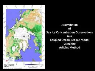
Assimilation of Sea Ice Concentration Observations in a Coupled Ocean-Sea Ice Model using the Adjoint Method
Section 1 Ocean-Sea ice state estimation using adjoint method
Methodology: Adjoint Method Ocean - Sea Ice State Estimation Goal is to generate a dynamical reconstruction of the three dimensional time-varying ocean-sea ice system : state estimate Essentially , model and observations are reconciled in a least-squares sense System evolves on the merits of the physics and thermodynamics encoded in the numerical model given initial and boundary conditions Iteratively adjust initial and boundary conditions using information provided by the Lagrange multipliers of the system, as provided by model adjoint. J. Gebbie 2004 Thesis Circle/bars : observations + uncertainties Solid : initial state trajectory Dashed : improved state estimate
Practical Lagrange Multipliers for Thermodynamic Sea Ice Model • Assume model is ice-free because of ocean has not yet been forced to the freezing point • Sea ice concentration observations • Proxy SST • Proxy upper ocean stratification • Proxy SST • Assume SST under sea ice is at the salinity determined freezing point • Effect is to change atm. state so as to increase air-sea heat fluxes and decrease initial thermal reservoir in the upper ocean • Proxy Stratification • Assume a well stratified ~ 50 m stratified mixed layer beneath ice, stratified by salinity • Effect is to modify initial and lateral open boundary ocean conditions. Information in the Lagrange multipliers is used to choose adjustments to model initial and boundary conditions so as to reduce model-data misfit Lagrange multipliers evolve through the ocean-ice adjoint model, which is itself driven by model-data misfit Thermodynamic sea ice model adjoint driven by sea ice concentration misfit Complications arise when an observation indicates sea ice but forward model trajectory is ice free. In this case the Lagrange multipliers evolving through the pure sea ice adjoint are zero.
Model, Initialization, and Boundary Forcing Ocean : 3-D prognostic Ocean Model (MITgcm) + KPP Mixed Layer Ice: Hibler VP + Semtner 0-Layer Ice Thermo + Snow Initial Condition Guess : ECCO ocean state estimate NCEP 6 hourly reanalysis (Fluxes calculated by model) Time Window : 1 year and 12 years ECCO SOLUTION Regional Domain
Section 2 Atmosphere-Ocean-Sea ICE Observations and their uncertainties
SSM/I MODIS : May 9, 1999 Sea Ice Observations Credit Provided by the SeaWiFS Project, NASA/Goddard Space Flight Center, and ORBIMAGE
in situ ocean observations [Sep 1996 -August 1997 ] Observation Locations Number of Observations with depth Temperature Uncertainty Blue = CTD Red = XBT Black = Profiling Floats (PALACE, ARGO, etc)
NCEP Reanalysis errors across the MIZ Observed near surface air temperature acoss marginal ice zone Reanalysis ice mask - SSM/I Ice Concentrations ~ 13o C Marginal Ice Zone NCEP Horiz. Res. Adapted from Renfrew et al 1999 (3/10/1992) 209 km
Section 3 Adjustments to model controls
Adjustments to NCEP Surface Air Temperature [Time Varying] σ=2.5oC 2σ • Adjustments compensate for errors in • Ocean-ice model and atmospheric • forcing errors • Reanalysis : Crude sea ice mask • Model : Unresolved MIZ eddy motion May 7-14, 2007
Eddy motion Image Credit NASA
Adjustments to NCEP Surface Air Temperature [Annual Bias] σ=1oC 2σ • Adjustments compensate for errors in • Ocean-ice model and atmospheric • forcing errors • Reanalysis : Warm Bias • Model : 1) WGC inflow too warm • 2) Incomplete penetration of WGC through Davis Strait
Section 4 Improvements On first-guess model trajectory
Improvement of Sea Ice Concentration[March 2004] Model Discrepancy Initial Guess Observation State Estimate > 73 iterations
State Estimate vs. Forward Model Run Feb 97 – Mar 97 Model Initial Guess MLD State Estimate MLD
State Estimate vs. Profiling Floats + CTD Feb 97 – Mar 97 Interpolated from CTD State Estimate MLD Pickard et al 2002
State Estimate vs. Profiling Floats + CTD Feb 97 – Mar 97 MLD from Floats + CTD State Estimate MLD : < 500 m : > 500 m < 1000 m : > 1000 m
Conclusions • Sea ice concentrations assimilated into ocean-Sea ice state estimate using the adjoint method • State estimate using ice and ocean observations in the Labrador Sea modifies NCEP reanalysis atmospheric state in ways which are consistent with estimated reanalysis errors • Inclusion of sea ice concentration leads to an state with significantly improved sea ice concentrations and mixed layer depths