Ocean State Estimation for Climate Research
220 likes | 390 Vues
Ocean State Estimation for Climate Research. Tong Lee, NASA JPL Toshiyuki Awaji, Kyoto University Magdalena Balmaseda, ECMWF Eric Greiner, CLS Detlef Stammer, Universität Hamburg. Three streams of GODAE efforts. Operational ocean analysis and forecast

Ocean State Estimation for Climate Research
E N D
Presentation Transcript
Ocean State Estimation for Climate Research Tong Lee, NASA JPL Toshiyuki Awaji, Kyoto University Magdalena Balmaseda, ECMWF Eric Greiner, CLS Detlef Stammer, Universität Hamburg GODAE Final Symposium, 12 – 15 November 2008, Nice, France
Three streams of GODAE efforts • Operational ocean analysis and forecast • (presentations by Hurlburt et al. & Kamachi et al.) • Initialization of seasonal-interannual prediction • (presentation by Balmaseda et al.) • State estimation for climate research • (this presentation) GODAE Final Symposium, 12 – 15 November 2008, Nice, France
Estimation Systems • Models: • MOMx, POP, MITOGCM, OPA/NEMO, etc. • Data constraints: • SSH, T/S profiles, SST, SSS, velocity data, … elephant-seal data. • Assimilation methods: • OI, 3D-VAR, Kalman filters (and smoother), adjoint (4D-VAR). • Presentations by Dombrowsky et al. by Cummings et al. for • further individual descriptions. GODAE Final Symposium, 12 – 15 November 2008, Nice, France
Science Applications • A large number of applications over a wide range of subjects (from physical oceanography & climate to biogeochemistry & geodesy). • Examples (physical oceanography related) • Meridional overturning circulation (MOC) • (e.g., Lee & Fukumori ‘03, Schoenefeldt & Schott ‘06, Schott et al. ‘07 & ‘08, • Wunsch & Heimbach ‘06, Balmadeda et al. ‘07, Cabanes et al. ‘08, Köhl & • Stammer ’08, Rabe et al. ‘08) • Water-mass pathways • (e.g., Fukumori et al. ‘04, Wang et al. ‘04, Masuda et al. ‘06, Toyoda et al. ‘08) • Heat budget • (e.g., Kim et al ‘04, ‘06, ‘07, Halkides & Lee ’08-a & ‘08-b) • Sea level (SSH) variability • (e.g., Carton et al. ‘05, Wunsch et al. ‘07, Köhl & Stammer ‘08) • Intercomparison GODAE Final Symposium, 12 – 15 November 2008, Nice, France
3-D structure of the anomalous subtropical cell (STC) of the Pacific Ocean Pacific Ocean STC Tradewind anomaly Conventional 2-D view via meridional transport stream function 10S 10N N Poleward Ekman flow Lower branch of the STC has a zonal structure characterized by anti-correlated anomalies of boundary & interior flows, thus opposite roles in regulating tropical heat content (Lee & Fukumori 2003, Schott et a. 2007) Equatorward thermocline flow Conventional bird’s eye view New view: 3-D structure Poleward Ekman flow Poleward Ekman flow LLWBC flow Equatorward thermocline flow Interior thermocline flow Poleward Ekman flow Poleward Ekman flow
How do satellite data help constrain estimates of the anti-correlated boundary & interior flows • Observed SSHA suggest local • recirculation in w. Pacific causing anti-correlated boundary & • interior flows (Lee & Fukumori • 2003, Lee & McPhaden 2008). • Need to monitor LLWBCs, which • are not well sampled by existing • in-situ systems. Trend of SSH 1993-2000 GODAE Final Symposium, 12 – 15 November 2008, Nice, France
Anti-correlated anomalies of boundary & interior flows in G-ECCO product Schott, Wang, & Stammer (2007) confirms finding of Lee & Fukumori (2003) (shorter period) 10°N 10°S GODAE Final Symposium, 12 – 15 November 2008, Nice, France
The North Atlantic Meridional Overturning Circulation (MOC) Picture from http://www.noc.soton.ac.uk GODAE Final Symposium, 12 – 15 November 2008, Nice, France
Interannual variation of N. Atl. MOC: mechanism & fingerprinting (Cabanes, Lee, and Fu 2008) • Interannual variation of MOC in subtropical N. Atl. is correlated with pycnocline depth difference Δh between west & east coasts • Δh variation dominated by W.B. (mainly due to near local wind) MOC anomaly at 1000 m Normalized time series (by std. dev.) Pycnocline depth difference across basin • ΔSSH is not indicative of subtropical N. Atl. MOC variation because of dominant steric contribution in the upper 200 m GODAE Final Symposium, 12 – 15 November 2008, Nice, France
Decadal change of N. Atl. MOC at 26N estimated by an ECCO-GODAE product (Wunsch & Heimbach 2006) • Complex vertical structure: • Weakening northward transport above 1000 m • Strengthening southward transport of NADW • Strengthening northward transport of abyssal water • No significant decrease of northward heat transport (upper-ocean warming enhances vertical temperature gradient to offset weakening of upper MOC). • Opposite trends of MOC strength at 26N & 50N. GODAE Final Symposium, 12 – 15 November 2008, Nice, France
Decadal change of N. Atl. MOC at 26N estimated by ECMWF ocean reanalysis product (Balmaseda, Smith, and Haines, et al. 2007) Assimilation improves comparison with observational analysis Cunningham et al. (2007) Bryden et al. (2005) • Large month-to-month variability and related uncertainty in model & data. • Complex structure of trends (both in vertically & meridionally). • Upper-ocean warming enhances vertical T gradient to offset weakening MOC. GODAE Final Symposium, 12 – 15 November 2008, Nice, France
Using passive tracer adjoint to study water-mass pathways Origin of “NINO-3” waters: Fukumori, Lee, Cheng, & Menemenlis 2004) • Other examples: • Wang et al. (2004): cause for interannual co-variability of T & S in the cold tongue. • Toyoda et al. (2008): interannual variation of subtropical Pacific mode water. Other GODAE Final Symposium, 12 – 15 November 2008, Nice, France
Global sea level rise in SODA ocean reanalysis (Carton, Giese, and Grodsky 2005) The apparent acceleration of sea level rise in1990s was explainable to by fluctuations in warming and thermal expansion of the oceans (upper 1000 m) Miller & Douglas 2004 Levitus et al. 2005 GODAE Final Symposium, 12 – 15 November 2008, Nice, France
Studying patterns of decadal trend (1993-2004) of SSH in an ECCO-GODAE product (Wunsch, Ponte, & Heimbach 2007) Zonal sums of trends in ρ (a), T (b) and S (c) over various depth ranges showing non-negligible contributions from below 850 m (a) (b) (c) Observational errors & potential impact on state estimation GODAE Final Symposium, 12 – 15 November 2008, Nice, France
Physically consistent state estimation allows budget closure – important to climate diagnostic analysis Mixed-layer temperature (MLT) budget: Kim, Lee, & Fukumori (2004): Ocean dynamics contributed to the mid-latitude warming significantly. N. Pac. SST warming during 1997-2000 Budget for MLT interannual anomaly GODAE Final Symposium, 12 – 15 November 2008, Nice, France
Intercomparison - climate time scales (presentation by Hernandez et al. for shorter time scales) • CLIVAR/GODAE global ocean reanalysis product evaluation: the ability to detect climate signals. • Many thanks to • various groups for providing a large number of indices & participate the discussion; • several analysts for performing the intercomparison; • APDRC/IPRC (Peter Hacker’s group) for assistance. • Examples … GODAE Final Symposium, 12 – 15 November 2008, Nice, France
Comparison for anomaly of ITF volume transport among 13 ocean reanalysis products (1993-2001) r.m.s. diff. 2 Sv r.m.s. diff. 1 Sv r.m.s. diff. 1 Sv
Statistics of ITF volume transport comparison for the 13 products (all in Sv) • Ensemble mean: 13.8 • r.m.s. difference of time mean: 3.7 • Averaged temporal variability (>monthly) of different products: 3.6 • r.m.s. difference of anomalies: 1 - seasonal, 2 - non-seasonal, 1 - interannual • r.m.s. diff. for time mean larger than that for anomaly. • “Signal-to-noise” ratio > 1 • Requirements for observational accuracy (e.g., from INSTANT observations) to distinguish different products (also have statistics for T & S fluxes).
S300: 1993-2002 S300: 1960-2002 T300:1993-2002 T300: 1960-2002 EQPAC EQATL EQINDTRPAC TRATL NPAC NATL GLOBAL How well do ocean reanalysis detect climate variability? --- Signal/Noise Ratio Signal/Noise ratio of upper 300m averaged T & S in various regions for 20 products (Balmaseda & Weaver 2008) GODAE Final Symposium, 12 – 15 November 2008, Nice, France
Time evolution & ensemble spread of upper 300m mean T & S for 20 products (Balmaseda & Weaver’08) The colored envelopes (or their differences) indicate the spread due to different forcing, model, or assimilation methods GODAE Final Symposium, 12 – 15 November 2008, Nice, France
Challenges ahead • Model physics • Model & data errors • Physical consistency for sequential/filter methods • Control space for adjoint & Green’s function methods • Coupled assimilation • Resources issues GODAE Final Symposium, 12 – 15 November 2008, Nice, France
Summary • Significant advancement in ocean state estimation for climate research has been achieved in the past decades. • Global ocean synthesis evaluation help identify pros & cons. • Ongoing challenges require sustained resources and effort & collaboration with a broader community. GODAE Final Symposium, 12 – 15 November 2008, Nice, France