Inferential Statistics
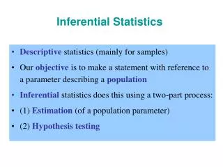
Inferential Statistics. Descriptive statistics (mainly for samples) Our objective is to make a statement with reference to a parameter describing a population Inferential statistics does this using a two-part process: (1) Estimation (of a population parameter) (2) Hypothesis testing.

Inferential Statistics
E N D
Presentation Transcript
Inferential Statistics • Descriptive statistics (mainly for samples) • Our objective is to make a statement with reference to a parameter describing a population • Inferential statistics does this using a two-part process: • (1) Estimation (of a population parameter) • (2) Hypothesis testing
Inferential Statistics • Estimation (of a population parameter) - The estimation part of the process calculates an estimate of the parameter from our sample (called a statistic), as a kind of “guess” as to what the population parameter value actually is • Hypothesis testing - This takes the notion of estimation a little further; it tests to see if a sampled statistic is really different from a population parameter to a significant extent, which we can express in terms of the probability of getting that result
Point Estimate x = Estimator n i=n S xi i=1 Estimation • Another term for a statistic is a point estimate, which is simply an estimate of a population parameter • The formula you use to compute a statistic is an estimator, e.g. • In this case, the sample mean is being used to estimate m, the population mean
Estimation • It is quite unlikely that our statistic will be exactly the same as the population parameter (because we know that sampling error does occur), but ideally it should be pretty close to ‘right’, perhaps within some specified range of the parameter • We can define this in terms of our statistic falling within some interval of values around the parameter value (as determined by our sampling distribution) • But how close is close enough?
Estimation and Confidence • We can ask this question more formally: • (1) How confident can we be that a statistic falls within a certain distance of a parameter • (2) What is the probability that the parameter is within a certain range that includes our sample statistic • This range is known as a confidence interval • This probability is the confidence level
Confidence Interval & Probability • A confidence interval is expressed in terms of a range of values and a probability (e.g. my lectures are between 60 and 70 minutes long 95% of the time) • For this example, the confidence level that I used is the 95% level, which is the most commonly used confidence level • Other commonly selected confidence levels are 90% and 99%, and the choice of which confidence level to use when constructing an interval often depends on the application
Central Limit Theorem • We have now discussed both the notions of probability and the way that the normal distribution • By combining these two concepts, we can go further and state some expectations about how the statistics that we derive from a sample might relate to the parameters that describe the population from which the sample is drawn • The approach that we use to construct confidence intervals relies upon the central limit theorem
The Central Limit Theorem • Suppose we draw a random sample of size n (x1, x2, x3, … xn – 1, xn) from a population random variable that is distributed with meanµ and standard deviationσ • Do this repeatedly, drawing many samples from the population, and then calculate the of each sample • We will treat the values as another distribution, which we will call the sampling distribution of the mean ( )
The Central Limit Theorem • Given a distribution with a mean μ and variance σ2, the sampling distribution of the mean approaches a normal distribution with a mean (μ) and a variance σ2/n as n, the sample size, increases • The amazing and counter- intuitive thing about the central limit theorem is that no matter what the shape of the original (parent) distribution, the sampling distribution of the mean approaches a normal distribution
Central Limit Theorem • A normal distribution is approached very quickly as n increases • Note that n is the sample size for each mean and not the number ofsamples • Remember in a sampling distribution of the mean the number of samples is assumed to be infinite • Foundation for many statistical procedures because the distribution of the phenomenon under study does not have to be normal because its average will be
Central Limit Theorem • Three different components of the central limit theorem • (1) successive sampling from a population • (2) increasing sample size • (3) population distribution • Keep in mind that this theorem applies only to the mean and not other statistics
Central Limit Theorem – Example • On the right are shown the resulting frequency distributions each based on 500 means. For n = 4, 4 scores were sampled from a uniform distribution 500 times and the mean computed each time. The same method was followed with means of 7 scores for n = 7 and 10 scores for n = 10. • When n increases:1. The distributions becomes more and more normal2. The spread of the distributions decreases Source: http://davidmlane.com/hyperstat/A14461.html
Central Limit Theorem – Example The distribution of an average tends to be normal, even when the distribution from which the average is computed is decidedly non-normal. Source: http://www.statisticalengineering.com/central_limit_theorem.htm
Central Limit Theorem & Confidence Intervals for the Mean • The central limit theorem states that given a distribution with a mean μ and variance σ2, the sampling distribution of the mean approaches a normal distribution with a mean (μ) and a variance σ2/n as n, the sample size, increases • Since we know something about the distribution of sample means, we can make statements about how confident we are that the true mean is within a given interval about our sample mean
s sX = n Standard Error • The standard deviation of the sampling distribution of the mean (X) is formulated as: • This is the standard error (the unit of measurement of a confidence interval, used to express the closeness of a statistic to a parameter • When we construct a confidence interval we are finding how many standard errors away from the mean we have to go to find the area under the curve equal to the confidence level
99.7% 95% 68% f(x) -3σ -2σ -1σμ+1σ+2σ +3σ P(Z>=2.0) = 0.0228 P(-2<=Z<=+2) = 1 – 2*0.0228 = 0.9544 P(Z>=1.96) = 0.025 P(-1.96<=Z<=+1.96) = 1 – 2*0.025 = 0.95
Confidence Intervals for the Mean • The sampling distributionof the mean roughly follows a normal distribution • 95% of the time, an individual sample mean should lie within 2 (actually 1.96) standard deviations of the mean
This tells us that 95% of the time the true mean should lie within of the sample mean Confidence Intervals for the Mean • An individual sample mean should, 95% of the time, lie within of the true mean, μ • Rearrange the expression:
Confidence Intervals for the Mean • More generally, a (1- α)*100% confidence interval around the sample mean is: • Where zα is the value taken from the z-table that is associated with a fraction αof the weight in the tails (and therefore α/2 is the area in each tail) margin of error Standard error
Example • Income Example: Suppose we take a sample of 75 students from UNC and record their family incomes. Suppose the incomes (in thousands of dollars) are: 28 29 35 42 ··· 158 167 235 Source: http://www.stat.wmich.edu/s160/book/node46.html
Example • We don't know σ so we can't use the interval! We will replace σ by the sample standard deviation s
Example (89.96 – 1.96*5.97, 89.96 + 1.96*5.97) (78.26, 101.66)
Constructing a Confidence Interval • 1. Select our desired confidence level (1-α)*100% • 2. Calculateαandα/2 • 3. Look up the corresponding z-score in a standard normal table • 4. Multiply the z-score by the standard error to find themargin of error • 5. Find the interval by adding and subtracting this product from the mean
Constructing a Confidence Interval - Steps • Select our desired level of confidence • Let’s suppose we want to construct an interval using the 95% confidence level • Calculate α and α/2 • (1-α)*100% = 95% α = 0.05, α/2 = 0.025 • 3. Look up the corresponding z-score • α/2 = 0.025 a z-score of 1.96
Constructing a Confidence Interval - Steps 4. Multiply the z-score by the standard error to find themargin of error 5. Find the interval by adding and subtracting this product from the mean
Common Confidence Levels and a values • For your convenience, here is a table of commonly used confidence levels, α and α/2 values, and corresponding z-scores: (1 - a)*100% αα/2 Zα/2 90% 0.1 0.05 1.645 95% 0.05 0.025 1.96 99% 0.01 0.005 2.58
Constructing a Confidence Interval - Example • Suppose we conduct a poll to try and get a sense of the outcome of an upcoming election with two candidates. We poll 1000 people, and 550 of them respond that they will vote for candidate A • How confident can we be that a given person will cast their vote for candidate A? • Select our desired levels of confidence • We’re going to use the 90%, 95%, and 99% levels
Constructing a Confidence Interval - Example • Calculate αand α/2 • Our a values are 0.1, 0.05, and 0.01 respectively • Our a/2 values are 0.05, 0.025, and 0.005 • 3. Look up the corresponding z-scores • Our Za/2 values are 1.645, 1.96, and 2.58 • Multiplythe z-score by the standard error to find the margin of error • First we need to calculate the standard error
Constructing a Confidence Interval - Example • Find the interval by adding and subtracting this product from the mean • In this case, we are working with a distribution we have not previously discussed, a normal binomial distribution (i.e. a vote can choose Candidate A or B, a binomial function) • We have a probability estimator from our sample, where the probability of an individual in our sample voting for candidate A was found to be 550/1000 or 0.55 • We can use this information in a formula to estimate the standard error for such a distribution:
s sX = n (0.55)(0.45) = = = 0.0157 1000 (p)(1-p) n Constructing a Confidence Interval - Example • Multiply the z-score by the standard error cont. • For a normal binominal distribution, the standard error can be estimated using: • We can now multiply this value by the z-scores to calculate the margins of error for each conf. level
Constructing a Confidence Interval - Example • Multiply the z-score by the standard error cont. • We calculate the margin of error and add and subtract that value from the mean (0.55 in this case) to find the bounds of our confidence intervals at each level of confidence: • MarginBounds • CI Za/2of error Lower Upper • 90% 1.645 0.026 0.524 0.576 • 95% 1.96 0.031 0.519 0.581 • 99% 2.58 0.041 0.509 0.591
t-distribution • The central limit theorem applies when the sample size is “large”, only then will the distribution of means possess a normal distribution • When the sample size is not “large”, the frequency distribution of the sample means has what is known as the t-distribution • t-distribution is symmetric, like the normal distribution, but has a slightly different shape • The t distribution has relatively more scores in its tails than does the normal distribution. It is therefore leptokurtic
t-distribution • The t-distribution or Student's t-distribution is a probability distribution that arises in the problem of estimating the mean of a normally distributed population when the sample size is small • It is the basis of the popular Student's t-tests for the statistical significance of the difference between two sample means, and for confidence intervals for the difference between two population means
t-distribution • The derivation of the t-distribution was first published in 1908 by William Sealy Gosset. He was not allowed to publish under his own name, so the paper was written under the pseudonym Student • The t-test and the associated theory became well-known through the work of R.A. Fisher, who called the distribution "Student's distribution" • Student's distribution arises when (as in nearly all practical statistical work) the population standard deviation is unknown and has to be estimated from the data
Confidence intervals & t-distribution • The areas under the t-distribution are given in Table A.3 in Appendix A • e.g., with a sample size of n = 30, 95% confidence intervals are constructed using t = 2.045, instead of the value of z = 1.96 used above for the normal distribution • For the commuting data (textbook):
Confidence intervals & t-distribution • We are 95% sure that the true mean is within the interval (16.54, 27.32) • More precisely, 95% of confidence intervals constructed from samples in this way will contain the true mean