Section 4.4 Sampling Distribution Models and the Central Limit Theorem
Section 4.4 Sampling Distribution Models and the Central Limit Theorem. Transition from Data Analysis and Probability to Statistics. Warmup. You really like red M&M’s. MARS Corp. says that of the millions of M&M’s they make each day, 20% are red.

Section 4.4 Sampling Distribution Models and the Central Limit Theorem
E N D
Presentation Transcript
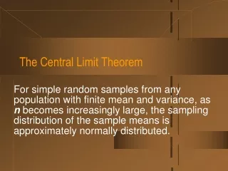
Section 4.4Sampling Distribution Models and the Central Limit Theorem Transition from Data Analysis and Probability to Statistics
Warmup • You really like red M&M’s. • MARS Corp. says that of the millions of M&M’s they make each day, 20% are red. • You purchase a large bag with 200 M&M’s (consider this a random sample of all M&M’s). • What is the probability that your bag has at least 48 red M&M’s?
Sampling Distribution Modelsfor Sample Proportions Sampling Distribution Modelsfor Sample Means OBJECTIVES At the conclusion of this unit you will be able to: • 1) Derive the correct sampling distribution model when given the population parameters • 2) Correctly apply the Central Limit Theorem to calculate probabilities associated with a sample proportion and sample mean
Probability: Statistics: From sample to the population (induction) • From population to sample (deduction)
Sampling Distributions • Population parameter: a numerical descriptive measure of a population. (for example: , p (a population proportion); the numerical value of a population parameter is usually not known) Example: = mean height of all NCSU students p=proportion of Raleigh residents who favor stricter gun control laws • Sample statistic: a numerical descriptive measure calculated from sample data. (e.g, x, s, p (sample proportion))
Parameters; Statistics • In real life parameters of populations are unknown and unknowable. • For example, the mean height of US adult (18+) men is unknown and unknowable • Rather than investigating the whole population, we take a sample, calculate a statistic related to the parameter of interest, and make an inference. • The sampling distribution of the statistic is the tool that tells us how close the value of the statistic is to the unknown value of the parameter.
DEF: Sampling Distribution • The sampling distribution of a sample statistic calculated from a sample of n measurements is the probability distribution of values taken by the statistic in all possible samples of size n taken from the same population. Based on all possible samples of size n.
Constructing a Sampling Distribution • In some cases the sampling distribution can be determined exactly. • In other cases it must be approximated by using a computer to draw some of the possible samples of size n and drawing a histogram.
Lecture Unit 4.4 Part 1 Sampling Distribution Models for Sample Proportions
Example: sampling distributionof p, the sample proportion • If a coin is fair the probability of a head on any toss of the coin is p = 0.5 (p is the population parameter) • Imagine tossing this fair coin 4 times and calculating the proportion p of the 4 tosses that result in heads (note that p = x/4, where x is the number of heads in 4 tosses). • Objective: determine the sampling distribution of p, the proportion of heads in 4 tosses of a fair coin.
Example: Sampling distribution of p There are 24 = 16 equally likely possible outcomes (1 =head, 0 =tail) (1,1,1,1) (1,1,1,0) (1,1,0,1) (1,0,1,1) (0,1,1,1) (1,1,0,0) (1,0,1,0) (1,0,0,1) (0,1,1,0) (0,1,0,1) (0,0,1,1) (1,0,0,0) (0,1,0,0) (0,0,1,0) (0,0,0,1) (0,0,0,0)
Sampling distribution of p (cont.) • E(p) =0*.0625+ 0.25*0.25+ 0.50*0.375 +0.75*0.25+ 1.0*0.0625 = 0.5 = p (the prob of heads) • Var(p) =
Expected Value and Standard Deviation of the Sampling Distribution of p • E(p) = p • SD(p) = where p is the “success” probability in the sampled population and n is the sample size
Shape of Sampling Distribution of p • The sampling distribution of p is approximately normal when the sample size n is large enough. n large enough means np ≥ 10 and n(1-p) ≥ 10
Shape of Sampling Distribution of p Population Distribution, p=.65 Sampling distribution of p for samples of size n
Example • 8% of American Caucasian male population is color blind. • Use computer to simulate random samples of size n = 1000
The sampling distribution model for a sample proportion p Provided that the sampled values are independent and the sample size n is large enough, the sampling distribution of p is modeled by a normal distribution with E(p) = p and standard deviation SD(p) = that is where n large enough means np>=10 and n(1-p)>=10 The Central Limit Theorem will be a formal statement of this fact.
Example: binge drinking by college students • Study by Harvard School of Public Health: 44% of college students binge drink. • 244 college students surveyed; 36% admitted to binge drinking in the past week • Assume the value 0.44 given in the study is the proportion p of college students that binge drink; that is 0.44 is the population proportion p • Compute the probability that in a sample of 244 students, 36% or less have engaged in binge drinking.
Example: binge drinking by college students (cont.) • Let p be the proportion in a sample of 244 that engage in binge drinking. • We want to compute • E(p) = p = .44; SD(p) = • Since np = 244*.44 = 107.36 and nq = 244*.56 = 136.64 are both greater than 10, we can model the sampling distribution of p with a normal distribution, so …
Example: snapchat by college students • recent scientifically valid survey : 77% of college students use snapchat. • 1136 college students surveyed; 75% reported that they use snapchat. • Assume the value 0.77 given in the survey is the proportion p of college students that use snapchat; that is 0.77 is the population proportion p • Compute the probability that in a sample of 1136 students, 75% or less use snapchat.
Example: snapchat by college students (cont.) • Let p be the proportion in a sample of 1136 that use snapchat. • We want to compute • E(p) = p = .77; SD(p) = • Since np = 1136*.77 = 874.72 and nq = 1136*.23 = 261.28 are both greater than 10, we can model the sampling distribution of p with a normal distribution, so …
Recall:Warmup • You really like red M&M’s. • MARS Corp. says that of the millions of M&M’s they make each day, 20% are red. • You purchase a large bag with 200 M&M’s (consider this a random sample of all M&M’s). • What is the probability that your bag has at least 48 red M&M’s?
Lecture Unit 4.4 Part 2 Sampling Distribution Modelsfor the Sample Mean x Continue the Transition from Data Analysis and Probability to Statistics
DEFINITION: Sampling Distribution • The sampling distribution of a sample statistic calculated from a sample of n measurements is the probability distribution of values taken by the statistic in all possible samples of size n taken from the same population. Based on all possible samples of size n.
Another Population Parameter of Frequent Interest: the Population Mean µ • To estimate the unknown value of µ, the sample mean x is often used. • We need to examine the Sampling Distribution of the Sample Mean x (the probability distribution of all possible values of x based on a sample of size n).
Example • Professor Stickler has a large statistics class of over 300 students. He asked them the ages of their cars and obtained the following probability distribution: x 2 3 4 5 6 7 8 p(x) 1/14 1/14 2/14 2/14 2/14 3/14 3/14 • SRS n=2 is to be drawn from pop. • Find the sampling distribution of the sample mean x for samples of size n = 2. Population values and their probability distribution
Solution • 7 possible ages (ages 2 through 8) • Total of 72=49 possible samples of size 2 • All 49 possible samples with the corresponding sample mean are on p. 48 in the coursepack and on the next slide.
All 49 possible samples of size n = 2 Population: ages of cars and their distribution x 2 3 4 5 6 7 8 p(x) 1/14 1/14 2/14 2/14 2/14 3/14 3/14
Probability Distribution of the Sample Mean Age of 2 Cars x 2 2.5 3 3.5 4 4.5 5 5.5 6 6.5 7 7.5 8 p(x)1/196 2/196 5/196 8/196 12/196 18/196 24/196 26/196 28/196 24/196 21/196 18/196 9/196
Solution (cont.) • Probability distribution of x: x 2 2.5 3 3.5 4 4.5 5 5.5 6 6.5 7 7.5 8 p(x) 1/196 2/196 5/196 8/196 12/196 18/196 24/196 26/196 28/196 24/196 21/196 18/196 1/196 • This is the sampling distribution of x because it specifies the probability associated with each possible value of x • From the sampling distribution above P(4 x 6) = p(4)+p(4.5)+p(5)+p(5.5)+p(6) = 12/196 + 18/196 + 24/196 + 26/196 + 28/196 = 108/196
Expected Value and Standard Deviation of the Sampling Distribution of x
Example (cont.) • Population probability dist. x 2 3 4 5 6 7 8 p(x) 1/14 1/14 2/14 2/14 2/14 3/14 3/14 • Sampling dist. of x x 2 2.5 3 3.5 4 4.5 5 5.5 6 6.5 7 7.5 8 p(x)1/196 2/196 5/196 8/196 12/196 18/196 24/196 26/196 28/196 24/196 21/196 18/196 1/196
Mean of sampling distribution of x: E(X) = 5.714 Population probability dist. x 2 3 4 5 6 7 8 p(x) 1/14 1/14 2/14 2/14 2/14 3/14 3/14 Sampling dist. of x x 2 2.5 3 3.5 4 4.5 5 5.5 6 6.5 7 7.5 8 p(x) 1/196 2/196 5/196 8/196 12/196 18/196 24/196 26/196 28/196 24/196 21/196 18/196 1/196 E(X)=2(1/14)+3(1/14)+4(2/14)+ … +8(3/14)=5.714 Population mean E(X)= = 5.714 E(X)=2(1/196)+2.5(2/196)+3(5/196)+3.5(8/196)+4(12/196)+4.5(18/196)+5(24/196) +5.5(26/196)+6(28/196)+6.5(24/196)+7(21/196)+7.5(18/196)+8(1/196) = 5.714
x 1 2 3 4 5 6 p(x) 1/6 1/6 1/6 1/6 1/6 1/6 Sampling Distribution of the Sample Mean X: Example • An example • A fair 6-sided die is thrown; let X represent the number of dots showing on the upper face. • The probability distribution of X is Population mean : = E(X) = 1(1/6) +2(1/6) + 3(1/6) +……… = 3.5. Population variance 2 2 =V(X) = (1-3.5)2(1/6)+ (2-3.5)2(1/6)+ ……… ………. = 2.92
Suppose we want to estimate m from the mean of a sample of size n = 2. • What is the sampling distribution of in this situation?
E( ) =1.0(1/36)+ 1.5(2/36)+….=3.5 V(X) = (1.0-3.5)2(1/36)+ (1.5-3.5)2(2/36)... = 1.46 6/36 5/36 4/36 3/36 2/36 1/36 1 1.5 2.0 2.5 3.0 3.5 4.0 4.5 5.0 5.5 6.0
Notice that is smaller than Var(X). The larger the sample size the smaller is . Therefore, tends to fall closer to m, as the sample size increases. 1 6 1 6 1 6
The variance of the sample mean is smaller than the variance of the population. Mean = 1.5 Mean = 2. Mean = 2.5 1.5 2.5 Population 2 1 2 3 1.5 2.5 2 1.5 2 2.5 1.5 2 2.5 1.5 2.5 Compare the variability of the population to the variability of the sample mean. 2 1.5 2.5 Let us take samples of two observations 1.5 2 2.5 1.5 2 2.5 1.5 2.5 2 1.5 2.5 1.5 2 2.5 1.5 2 2.5 1.5 2 2.5 Also, Expected value of the population = (1 + 2 + 3)/3 = 2 Expected value of the sample mean = (1.5 + 2 + 2.5)/3 = 2
µ Unbiased Unbiased Confidence l Precision l The central tendency is down the center BUS 350 - Topic 6.1 6.1 - 14 Handout 6.1, Page 1