Download
1 / 14
140 likes | 379 Vues
REVIEW Central Limit Theorem and The t Distribution. Random Variables. A random variable is a quantitative “experiment” whose outcome is not known in advance. All random variables have three things: A distribution A mean A standard deviation. _ The Random Variables X and X.

E N D
REVIEW Central Limit Theorem and The t Distribution
Random Variables A random variable is a quantitative “experiment” whose outcome is not known in advance. All random variables have three things: • A distribution • A mean • A standard deviation
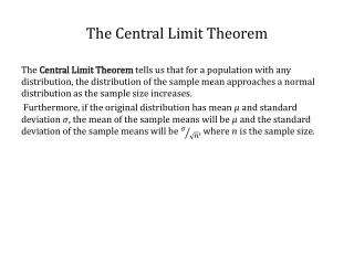
_The Random Variables X and X X = a random variable designating the outcome of a single event Mean of X = µ; Standard deviation of X = σ _ X = a random variable designating the average outcome of n measurements of the event _ _‗Mean of X = µ; Standard deviation of X = σ/√n THIS IS ALWAYS TRUE AS LONG AS σ IS KNOWN!
Example Attendance at a basketball game averages 20000 with a standard deviation of 4000. X = Attendance at a game µ = 20000; σ= 4000 _ X = Average attendance at n games _ Mean of X = 20000 ‗ ‗ Standard deviation of X = 4000/√n
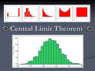
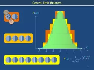
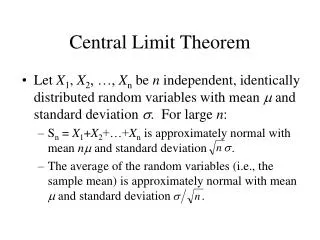
The Central Limit Theorem 1 2 Central Limit Theorem • Assume that the standard deviation of the random variable X, σ, is known. • Two cases for the distribution of X X (Attendance at a game) is normal. THEN _ X (Average attendance at n games) has a normal distribution for any sample size, n X (Attendance at a game) is not normal. THEN _ X (Average attendance at n games) has an unknown distribution. But the larger the value of n, the closer it is approximated by a normal distribution.
What is a Large Enough Sample Size? • _ To determine whether or not X can be approximated by a normal distribution, typically n = 30 is used as a breakpoint. • In most cases, smaller values of n will provide satisfactory results, particularly if the random variable X (attendance at a game) has a distribution that is somewhat close to a normal distribution.
Examples Attendance at a basketball game averages 20000 with a standard deviation of 4000. • Assuming that attendance at a game follows a normal distribution, what is the probability that: • Attendance at a game exceeds 21000? • Average attendance at 16 games exceeds 21000? • Average attendance at 64 games exceeds 21000? • Repeat the above when you cannot assume attendance follows a normal distribution.
Answers Assuming Attendance Has a Normal Distriubtion • If X, attendance, has a normal distribution since σ is known to = 4000, THEN • _ Average attendance, X, is normal with: ‗ Standard deviation of X = __ 4000/√16 = 1000 in case 2 and __ 4000 /√64 = 500 in case 3.
Calculations • Case 1: P(X > 21000) Here, z = (21000-20000)/4000 = .25 So P(X > 21000) = 1 - .5987 = .4013 • _ Case 2: P(X > 21000) Here, z = (21000-20000)/1000 = 1.00 _ So P(X > 21000) = 1 - .8413 = .1587
Calculations (Continued) • _ Case 3: P(X > 21000) Here, z = (21000-20000)/500 = 2.00 _ So P(X > 21000) = 1 - .9772 = .0228
Answers Assuming Attendance Does Not Have a Normal Distriubtion • Case 1 : Since X is not normal we cannot evaluate P(X > 21000) • _ Case 2: Since X is not normal, n is small, X has an unknown distribution. Thus we cannot evaluate this probability either. • Since n is large, case 3 can be evaluated in the same manner as when X was assumed to be normal: _ Case 3: P(X > 21000) Here, z = (21000-20000)/500 = 2.00 _ So P(X > 21000) = 1 - .9772 = .0228
What Happens When σ Is Unknown? -- t Distribution • This is the usual case. _ • If X has a normal distribution, X will have a t distribution with: • n-1 degrees of freedom _ • Standard deviation = s/√n • But the t distribution is “robust” meaning we can use it even when X is only roughly normal – a common assumption. • From the central limit theorem, it can also be used with large sample sizes when σ is unknown.
When to use z and When to use t • USEz • Large n or sampling from a normal distribution • σ is known • USEt • Large n or sampling from a normal distribution • σ is unknown • z and t distributions are used in hypothesis testing and confidence intervals _ These are determined by the distribution of X.
REVIEW _ • The random variables X and X • Mean and standard deviation • Central Limit Theorem _ • Probabilities For the Random Variable X • t Distribution • When to use z and When to Use t • Depends only on whether or not σ is known