Download
1 / 8
120 likes | 338 Vues
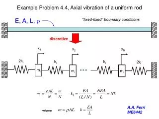
Example Problem 4.4, Axial vibration of a uniform rod. E, A, L, r. “fixed-fixed” boundary conditions. discretize. x 1. x 2. x N. 2k i. k i. k i. 2k i. m i. m i. m i. A.A. Ferri ME6442. where. Mass and stiffness matrices. Characteristic Equation:. Define:.

E N D
Example Problem 4.4, Axial vibration of a uniform rod E, A, L, r “fixed-fixed” boundary conditions discretize x1 x2 xN 2ki ki ki 2ki mi mi mi A.A. Ferri ME6442 where
Mass and stiffness matrices Characteristic Equation: Define:
Matlab Implementation N=50; d_main=2*ones(1,N); d_sub = -ones(1,N-1); K=diag(d_main) + diag(d_sub,1) + diag(d_sub,-1); K(1,1)=3; K(N,N)=3; Kprime = N*K; M=eye(N); Mprime=M/N; “super-diagonal” “sub-diagonal” overwrite 1st and Nth entries on main diagonal [phi,lam]=eig(Kprime,Mprime); wn=sqrt(diag(lam)); % N=10 gives: % wn' = [3.1287 6.1803 9.0798 11.7557 14.1421 % 16.1803 17.8201 19.0211 19.7538 20.0000]
mu_mat = phi'*Mprime*phi; % for N = 10, off diag terms of mu_mat % are order 3.5e-016 mu = diag(mu_mat); PHI=zeros(N,N); % Normalize modes for j=1:N; PHI(:,j)=phi(:,j)/sqrt(mu(j)); end; % plot modeshapes figure(1) plot(1:N,PHI(:,1),'o-',1:N,PHI(:,2),'^-') xlabel('DOF #'); ylabel('Modes 1 and 2') legend('Mode 1','Mode 2')
Comparison of exact vs approximate natural frequencies, N = 50
% error in approximate natural frequencies, N = 50 For N = 50, we get 50 natural frequencies, but only the first 25 are accurate to within 10%