Download

1 / 61
610 likes | 768 Vues
Learn the basics of nodal pricing in electricity markets, including locational differences, impedance effects on power flow, loss comparison, and security limits. Explore examples and calculations to grasp how nodal prices are determined for efficient market operation.

E N D
Nodal Pricing Basics Drew Phillips Market Evolution Program 1
Agenda • What is Nodal Pricing? • Impedance, Power Flows Losses and Limits • Nodal Price Examples • No Losses or Congestion • Congestion Only • Impact of Transmission Rights • Losses Only • How DSO Calculates Nodal Prices 2
What is Nodal Pricing? • Nodal Pricing = Locational Marginal Pricing (LMP) = Locational Based Marginal Pricing (LBMP) • Nodal Pricing is a method of determining prices in which market clearing prices are calculated for a number of locations on the transmission grid called nodes • Each node represents the physical location on the transmission system where energy is injected by generators or withdrawn by loads • Price at each node represents the locational value of energy, which includes the cost of the energy and the cost of delivering it, i.e., losses and congestion • IMO publishes nodal prices for information purposes; they are referred to as shadow prices 3
What causes locational differences? Losses • Due to the physical characteristics of the transmission system, energy is lost as it is transmitted from generators to loads • Additional generation must be dispatched to provide energy in excess of that consumed by load • Transmission congestion • Prevents lower cost generation from meeting the load; higher cost generation must be dispatched in its place • In both cases, the associated costs are allocated to each node in a manner that recognizes their individual contribution to/impact on these extra costs 4
Impedance and its effect on power flows Impedance • Is a characteristic of all transmission system elements • Signifies opposition to power flow • A higher impedance path indicates more opposition to power flow and greater losses Impedance between two points on the grid is related to: • Line length • Number of parallel paths • Voltage level • Number of series elements such as transformers Impedance will be lower where there are: • Shorter transmission lines • More parallel paths • Higher voltage • Fewer series transformers 6
230 kV Gen 115 kV Load Relative Impedance and Power Flow Transformer • Energy will flow preferentially on the 230 kV path: • Higher voltage • More lines in parallel • Fewer transformers 7
Power Flows • Power will take all available paths to get from supply point to consumption point • Power flow distribution on a transmission system is a function of: • Location and magnitude of generation • Location and magnitude of load • Relative impedance of the various paths between generation and load • The following examples ignore the effect of losses 8
75 % W Gen 25 % S W E N Power Flows N Load • All lines have equal impedance • Path W-S-E-N has three times the impedance of path W-N • Flow divides inversely to impedance • If W Gen supplies N Load, flow W-S-E-N is one third flow W-N • If N Load is 100 MW, 75 MW flows on path W-N, 25 MW flows on path W-S-E-N E Gen 9
75 % 25 % S W E N What if E Gen supplies N Load? N Load • Path E-S-W-N has three times the impedance of path W-N • Flow divides inversely to impedance • If E Gen supplies N Load, flow E-S-W-N is one third flow E-N • If N Load is 100 MW, 75 MW flows on path E-N, 25 MW flows on path E-S-W-N E Gen 10
N Load 45 MW (15 +30) 55 MW 45 MW (45 +10) 30 MW E Gen 40 MW 60 MW W Gen 10 MW (15 –10) 5 MW 5 MW (15 –10) 15 MW S W E N Superposition 100 MW • What if W Gen supplies 60 MW and E Gen supplies 40 MW to N Load? • Both W Gen and E Gen’s output will flow in proportion to the impedance of the paths to N Load • Resulting line flows represent the net impact of their flow distribution 60 MW 60 MW 40 MW 11
79.5 MW 88.5 MW 89.9 MW 90 MW 90 MW 90 MW 180 A 390 A 780 A A 500 kV 230 kV 115 kV Loss Comparison for 100 km Lines Current (Amps) • Losses are: • proportional to Current2 x Resistance (I2R) • lower on higher voltage lines because resistance is lower and current flow is lower for a given MW flow 12
Loss Comparison • Losses are higher on a line that is heavily loaded for the same increase in current = 13
Security Limits • Security limits are the reliability envelope in which the market operates • Power will take all available paths to get from supply point to consumption point • Transmission lines do not control or limit the amount of power they convey • Power flows are managed by dispatching the system (normally via dispatch instructions and interchange scheduling) • Must respect current conditions and recognized contingencies 14
Marginal Cost of Transmission Congestion Nodal Price Marginal Cost of Generation Marginal Cost of Losses = + + How are nodal prices derived? • Marginal cost is the cost of the next MW; the marginal generator is the generator that would be dispatched to serve the next MW • This is the basis of our current unconstrained market clearing price • A nodal price is the cost of serving the next MW of load at a given location (node) • Nodal prices are formulated using a security constrained dispatch and the costs of supply are based upon participant offers and bids • Nodal prices consist of three components: 16
$ Uniform Price • Unconstrained • Calculation • ignores physical • limitations Market Schedule Market Participants IMO Bids/ Offers CMSC Bids/ Offers • Constrained • Calculation • considers physical • limitations Dispatch Schedule Dispatchable resources produce or consume MWs Current Pricing Scheme Nodal Prices Currently calculated for information purposes only 17
Nodal Price Calculations • No Congestion or Losses • With Congestion • With Losses Process: • Determine least cost dispatch to serve load • Determine resulting power flows to ensure security limits are respected • Calculate prices by determining the dispatch for one additional MW at each node (while still respecting all limits) 18
25 MW Offer Offer E Gen E Gen 125 @ $35 125 @ $30 W Gen Dispatch Dispatch 25 MW 75 MW 25 MW 100 MW 0 MW S W E N No Congestion or Losses: Dispatch N Load 100 MW Transmission Limit = 85 MW • Least cost solution would have W Gen supply all 100 MW to N Load, based on W Gen’s offer price • Resultant flow is within limits • Nodal price is the cost of serving the next MW • What are the prices at each node? 20
75.75 MW 25.25 MW (75 + .75) (25 + .25) Offer Offer E Gen E Gen 125 @ $30 125 @ $35 W Gen Dispatch Dispatch 25.25 MW 25.25 MW 100 MW 0 MW (25 + .25) (25 + .25) +1 MW S W E N No Congestion or Losses: Node N Price N Load 100 MW + 1 MW Transmission Limit = 85 MW • Price at Node N is the cost of supplying next 1 MW to N • Least cost solution would have W Gen supply the next MW to N, based on W Gen’s offer price • Resultant flow would be within limits (net of existing flow and increment to serve additional 1 MW at Node N) • W Gen is the marginal generator and Node N price = $30 $30 21
75 MW 25 MW Offer Offer E Gen E Gen 125 @ $30 125 @ $35 W Gen Dispatch Dispatch 25 MW 25 MW 0 MW 100 MW +1 MW S W E N No Congestion or Losses: Node W Price N Load 100 MW Transmission Limit = 85 MW • Price at Node W is the cost of supplying next 1 MW at W • Least cost solution would have W Gen supply the next MW to W, based on W Gen’s offer price • Resultant flow would be within limits (net flow change is zero) • W Gen is the marginal generator and Node W price = $30 + 1 MW $30 22
75.5 MW 24.5 MW (75 + .5) (25 - .5) Offer Offer E Gen E Gen 125 @ $35 125 @ $30 W Gen Dispatch Dispatch 25.5 MW 25.5 MW 100 MW 0 MW (25 + .5) (25 + .5) +1 MW S W E N No Congestion or Losses: Node E Price N Load 100 MW Transmission Limit = 85 MW • Price at Node E is the cost of supplying next 1 MW to E • Least cost solution would have W Gen supply the next MW to N, based on W Gen’s offer price • Resultant flow would be within limits (net of existing flow and increment to serve additional 1 MW at Node E) • W Gen is the marginal generator and Node E price = $30 + 1 MW $30 23
75.25 MW 24.75 MW (75 + .25) (25 - .25) Offer Offer E Gen E Gen 125 @ $35 125 @ $30 W Gen Dispatch Dispatch 25.75 MW 24.75 MW 100 MW 0 MW (25 - .25) (25 + .75) +1 MW S W E N No Congestion or Losses: Node S Price N Load 100 MW Transmission Limit = 85 MW • Price at Node S is the cost of supplying next 1 MW at S • Least cost solution would have W Gen supply the next MW to S, based on W Gen’s offer price • Resultant flow would be within limits (net of existing flow and increment to serve additional 1 MW at Node S) • W Gen is the marginal generator and Node S price = $30 $30 + 1 MW 24
Summary • The previous examples demonstrate the method used to derive nodal prices • As we would expect, the nodal prices at all nodes on a transmission system will be the same in the absence of losses and congestion • Unfortunately, no such transmission system exists • The following examples will apply the same method to illustrate the calculation under conditions of congestion and then losses • Examples: • are not representative of how the IMO-controlled grid is dispatched and therefore the impact on nodal prices is entirely fictitious; these scenarios were designed to illustrate a concept while keeping the calculation as simple as possible • are for illustrative purposes only and do not imply a settlement basis for a nodal pricing methodology for Ontario 25
25 MW Offer Offer E Gen E Gen 125 @ $35 125 @ $30 W Gen Dispatch Dispatch 25 MW 75 MW 25 MW 100 MW 0 MW S W E N Congestion (No Losses): Dispatch N Load 100 MW Transmission Limit = 75.2 MW • Assume the transmission limit is reduced; dispatch can be solved as in the no congestion case, but what is the effect on nodal prices? 27
75.2 MW 25.8 MW Offer Offer E Gen E Gen 125 @ $35 125 @ $30 W Gen Dispatch Dispatch 24.7 MW 24.7 MW 0 MW 100 MW -.1 MW +1.1 MW S W E N Congestion (No Losses): Node N Price N Load 100 MW + 1 MW Transmission Limit = 75.2 MW • An increase in output of 1 MW by either W Gen or E Gen alone will increase the W-N line flow over the limit; we must redispatch the system using both generators • If we reduce W Gen output by 0.1 MW (75% of the reduction will appear on W to N flow) and increase E Gen output by 1.1 MW (25% flows from N to W), net effect is on line W-N is a flow increase of .2 MW • This is the lowest cost way to meet an additional 1 MW at N • Node N price = $35.50 (1.1 X $35 – 0.1 X $30) $35.50 28
75.2 MW 24.8 MW Offer Offer E Gen E Gen 125 @ $35 125 @ $30 W Gen Dispatch Dispatch 25.2MW 25.2 MW 100 MW 0 MW +.6 MW +.4 MW S W E N Congestion (No Losses): Node E Price N Load 100 MW Transmission Limit = 75.2 MW • An increase in output of 1 MW by either W Gen or E Gen alone will increase the W-N line flow over the limit; we must redispatch the system using both generators • If we increase W Gen output by 0.4 MW (75% flows from W to N) and increase E Gen output by .6 MW (0% flows from N to W), net effect is on line W-N is a flow increase of .2 MW • This is the lowest cost way to meet an additional 1 MW at E • Node E price = $33 (0.6 X $35 + 0.4 X $30) + 1 MW $33 29
75.2 MW 24.8 MW Offer Offer E Gen E Gen 125 @ $30 125 @ $35 W Gen Dispatch Dispatch 25.6MW 24.6 MW 0 MW 100 MW +.2 MW +.8 MW S W E N Congestion (No Losses): Node S Price N Load 100 MW Transmission Limit = 75.2 MW • An increase in output of 1 MW by either W Gen or E Gen alone will increase the W-N line flow over the limit; we must redispatch the system using both generators • If we increase W Gen output by 0.8 MW (75% flows from W to N) and increase E Gen output by .2 MW (25% flows from N to W), net effect is on line W-N is a flow increase of .2 MW • This is the lowest cost way to meet an additional 1 MW at E • Node S price = $31 (0.2 X $35 + 0.8 X $30) $31 + 1 MW 30
75 MW 25 MW Offer Offer E Gen E Gen 125 @ $30 125 @ $35 W Gen Dispatch Dispatch 25 MW 25 MW 0 MW 100 MW +1 MW S W E N Congestion (No Losses): Node W Price N Load 100 MW Transmission Limit = 75.2 MW • Least cost solution would have W Gen supply the next MW to W, based on W Gen’s offer price • W Gen can meet the additional MW at Node W without affecting the transmission system (net flow change is zero) • W Gen is the marginal generator and Node W price = $30 + 1 MW $30 31
25 MW Offer Offer E Gen E Gen 125 @ $30 125 @ $35 W Gen Dispatch Dispatch 25 MW 75 MW 25 MW 0 MW 100 MW S W E N Congestion (No Losses): Summary N Load 100 MW Transmission Limit = 75.2 MW • System is congested on line W-N • Combination of W Gen and E Gen redispatch is necessary to meet incremental loads at Node N,E and S • If W Gen and N Load are settled at their respective nodal prices, the difference will result in a settlement surplus • Surplus due to the congestion component of different nodal prices is used to fund transmission rights $35.50 $30 $33 $31 32
Transmission Rights • Provide a hedge against congestion charges between two locations • Transmission rights holders receive the difference in congestion charges between the two locations defined by the transmission right • Using our example: • Price at N - Price at W = Congestion Charge • $35.5 - $30 = $5.50/MW • If N load holds 100 MW of transmission rights, they will receive 100 x $5.50 = $550 • N Load: • Pays 100 x $35.50 = $3550 for energy • Receives 100 x $5.50 = $550 for transmission rights • Net = $3000 • W Gen is paid 100 x $30 = $3000 33
Offer Offer E Gen E Gen 125 @ $35 125 @ $30 W Gen Dispatch Dispatch 25 MW 75 MW 0 MW 100 MW S W E N Exercise One N Load 100 MW • Assume the transmission limit is on line S-E (for simplicity we’ll allow flow to equal the limit, although in reality flow must be less than the limit) • The load at N is being served by W Gen with flows on the transmission system as shown • What are the nodal prices at N and S? 25 MW 25 MW Transmission Limit = 25 MW 34
(75 +.375 +.125) 75.5 MW 25.5 MW (25 +.125 +.375) Offer Offer E Gen E Gen 125 @ $30 125 @ $35 W Gen Dispatch Dispatch 25 MW 25 MW 0 MW 100 MW (25 +.125 –.125) (25 +.125 –.125) +.5 MW +.5 MW S W E N Exercise Answer: Node N Price N Load 100 MW + 1 MW • W Gen cannot be used as sole supply as any increase in output will increase the S-E line flow; must redispatch the system • Must increase W Gen output by 0.5 MW (25% flows from S to E) and increase E Gen output by 0.5 MW (25% flows from E to S) • Resultant flow would be within limits • Node N price = $32.50 (0.5 X $35 + 0.5 X $30) $32.50 Transmission Limit = 25 MW 35
(75 + .75) 75.25 MW 24.75 MW (25 - .25) Offer Offer E Gen E Gen 125 @ $30 125 @ $35 W Gen Dispatch Dispatch 25.75 MW 24.75 MW 100 MW 0 MW (25 - .25) (25 + .75) +1 MW S W E N Exercise Answer: Node S Price N Load 100 MW • W Gen can be used as sole supply; the increase in output to serve Node S will decrease the S-E line flow • Increase W Gen output by 1.0 (75% flows from E to S) • Resultant flow would be within limits • Node S price = $30 $30 + 1 MW Transmission Limit = 25 MW 36
75 MW Offer Offer E Gen E Gen 125 @ $35 125 @ $30 W Gen Dispatch Dispatch 0 MW 104 MW S W E N Losses (No Congestion): Dispatch N Load 100 MW • Least cost solution would have W Gen supply all 100 MW to N Load due to its lower offer price, but due to losses must generate 104 MW • Resultant flow is within limits • Nodal price is the cost of serving the next MW • What are the prices at Node N? 25 MW 78 MW 26 MW 38
Offer Offer E Gen E Gen 125 @ $35 125 @ $30 W Gen Dispatch Dispatch 0 MW 104 MW +1.04 MW S W E N Losses (No Congestion): Node N Price N Load 101 MW • Price at node N is the cost of supplying next 1 MW • W Gen must generate an additional 1.04 MW to N to deliver 1 MW at Node N • Resultant flow would be within limits • Node N price = $31.20 (1.04 X $30) • Prices at Nodes E and S would be similarly calculated • Price at Node W = $30 as an increment of load can be supplied from W Gen with no impact to transmission flows 75.75 MW 25.25 MW $31.20 78.9 MW 26.3 MW 39
Summary • When more than one generator is on the margin, prices may be: • higher than any offer • lower than any offer (and could even be negative) For additional examples see the Market Evolution Day Ahead Market web page and in particular: http://www.theimo.com/imoweb.pubs/consult/mep/dam_wg_2003sep16_LMPexamples.pdf • Even when there is no congestion on the transmission system directly connecting them, prices may be different between two nodes due to: • losses and/or • their differing impact on congested paths elsewhere in the system • If a generator is partially dispatched: nodal price = offer price • If a generator is fully dispatched: nodal price > than offer price • If a generator is not dispatched: nodal price < than offer price 40
How the Dispatch Scheduling Algorithm (DSO) Calculates Nodal Prices 41
Dispatch Scheduling Optimizer (DSO) • Two methods are available to calculate nodal prices: 1) calculate nodal prices at each node directly (as in previous examples) 2) calculate a reference node price then derive prices at all other nodes • The DSO uses method 2 as it requires less computing power and is faster: • It yields the same results as method 1 • It does not matter which node is chosen as the reference bus 42
Nodal Price Cost of losses incurred for the next MW of load at the node Σ αnk*μk λs (DFn - 1)* λs λn Cost of transmission limits incurred for the next MW of load at the node System Marginal Cost at Reference Node Calculate Nodal Prices Marginal Cost of Generation Marginal Cost of Losses Marginal Cost of Transmission Congestion LMP = + + 43
Inputs • Offers and bids • Forecast demand for the next interval based upon a snapshot of current demand modified by the expected +/- in the next interval • Load profile based upon the current system snapshot • Physical model of the transmission system • Security limits • Penalty Factors (losses) • represent losses between nodes and the reference bus • IMO uses fixed losses for each node based on historical power flows 44
Penalty Factors Load Z Non-dispatchable PF = 1.3 = 23% losses • Represent incremental impact on losses for generation or load at each node based on a representative power flow distribution on the grid • If PF > 1: losses are incurred for each MW delivered to Richview • If PF < 1: losses are reduced for each MW delivered to Richview PF = .97 = - 3.1% losses Gen D Richview Gen A Gen C Gen B PF = .9 = - 11.2% losses PF = .95 = - 5.3% losses PF = 1.01 = 1% losses 45
Penalty Factors • Penalty Factors • Bids and Offers • Richview Nodal Price • Forecast Load • Congestion Impact • System Limits • Transmission Model • Load Profile • Richview Nodal Price • All Other Nodal Prices • Congestion Impact • Dispatch Instructions Nodal Price Calculation in DSO DSO Calculation 1 DSO Calculation 2 46
Richview Equivalent Offer/Bid Stack Delivery Point Offer/Bid Stack Gen B 100 MW @ $70.7 Gen A 100 MW @ $75 .90 Gen A 100 MW @ $67.5 Gen B 100 MW @ $70 1.01 Gen D 100 MW @ $65 Gen C 100 MW @ $60 .95 Gen C 100 MW @ $57 Gen D 100 MW @ $50 1.3 Reference Bus Merit Order Penalty Factors Subsequent calculation addresses quantity differences due to the effect of losses 47
Effective Price Penalty Factors Richview Equivalent Offer/Bid Stack Delivery Point Offer/Bid Stack Gen D 100 MW @ $50 1.3 Gen D 100 MW @ $65 If we generate 100 MW at Gen D, only 100/1.3 or 76.9 MW shows up at Richview due to losses 100 MW at Gen D costs 100 x $50 = $5,000, which only yields 76.9 MW at Richview, resulting in an effective price of $5000/76.9 MW = $65 /MW 48
Determine Unconstrained Economic Solution Richview Equivalent Offer/Bid Stack Current system demand +/- forecast change in next interval Gen B 100 MW @ $70.7 Gen A 100 MW @ $67.5 Gen D 100 MW @ $65 Forecast Demand Gen C 100 MW @ $57 49
Gen D Gen A Gen C Gen B Introduce Physical Network Load Z • Allocate forecast demand to nodes based on load profile of current system • Run load flow to solve power balance using offers and bids at appropriate nodes, physical characteristics of transmission system and system limits • Determine System Marginal Cost at Richview 4% 3% 2% 5% 4% 1% 3% Richview 6% 2% 5% 4% 10% 50