Chapter 9 Shortest Paths and Discrete Dynamic Programming
Chapter 9 Shortest Paths and Discrete Dynamic Programming. Example 9.1 Littleville.

Chapter 9 Shortest Paths and Discrete Dynamic Programming
E N D
Presentation Transcript
Example 9.1 Littleville Suppose that you are the city traffic engineer for the town of Littleville. Figure 9.1(a) depicts the arrangement of one- and two-way streets in a proposed improvement plan for Littleville’s downtown, including the estimated average time in seconds that a car will require to transit each block. From survey and other data we can estimate how many driver trips originate at various origin points in the town, and the destination for which each trip is bound. But such survey data cannot indicate what streets will be selected by motorists to move from origin to destination in a street network that does not yet exist.
Example 9.1 Littleville One of the tasks of a traffic engineer is to project the route that drivers will elect, so that city leaders can evaluate whether flows will concentrate where they hope. A good starting point is to assume that drivers will do the most rational thing-follow the shortest time path from their origin to their destination. We need to compute all such shortest paths.
Example 9.1 Littleville 20 18 18 12 36 32 25 28 28 18 21 30 40 49 13 38
Example 9.1 Littleville 20 18 10 8 6 7 5 4 3 2 1 9 12 18 36 32 25 28 18 28 21 30 40 49 13 38
9.1 Shortest Path Models • Urban traffic, Satellite communications, or surface of a microchip. • Mathematical graphs model travel, flow, and adjacency patterns in a network. [9.1] • The nodes or vertices of a graph represent entities, intersections, and transfer points of the network. [9.2] • The arcs of a graph model available directed (one-way) links between nodes. Edges represent undirected (two-way) links. [9.3]
9.1 Shortest Path Models • A path is a sequence of arcs or edges connecting two specified nodes in a graph. Each arc or edge must have exactly one node in common with its predecessors in the sequence, any arcs must passed in the forward direction, and no node may be visited more than once. [9.4]
Shortest Path Problems • Shortest path problems seek minimum total length paths between specified pairs of nodes in a graph. [9.5]
Example 9.1 Littleville 20 • Name: Littleville • Graph: arcs and edges • Costs: nonnegative • Output: shortest paths • Pairs: all nodes to all others 18 10 2 8 5 6 1 9 4 3 7 12 18 36 25 28 18 28 21 40 49 13 38
Example 9.2 Texas Transfer Texas Transfer, a major trucker in the southwest, ships goods from its hub warehouse in Ft. Worth to all the cities shown. Trucks leave the hub and proceed directly to their destination city, with no intermediate dropoffs or pickups. Texas Transfer drivers are allowed to choose their own route from Ft. Worth to their destination. However, management’s proposal in current labor negotiations calls for drivers to be paid on the basis of shortest standard mileage to the location. That is, they will be paid according to the length of the shortest path from Ft. Worth to their destination city in the network of Figure 9.3. To see the impact of this proposal, we need to compute such shortest path distances for all cities.
Example 9.2 Texas Transfer Notice that the character of this shortest path task differs significantly from the Littleville example. Here we need only optimal path lengths, not the paths themselves. Also, we need shortest path lengths for only one origin or source—the Ft. Worth hub.
Example 9.2 Texas Transfer Amarillo • Name: Texas Transfer • Graph: edges only • Costs: nonnegative • Output: shortest path lengths • Pairs: one node to all others 359 Ft. Worth 122 Lubbock 10 5 4 9 7 1 3 8 2 6 180 167 Abilene 195 246 345 92 443 Austin Houston San Angelo 79 415 199 213 El Paso San Antonio 215 153 Corpus Christi
Example 9.3 Two Ring Circus The Two Ring Circus is nearing the end of its season and planning a return to winter headquarters near Tallahassee, Florida. Present commitments will end in Lincoln, Nebraska, but there are still some opportunities for bookings in cities along the route home. Figure 9.4(a) shows the travel routes available and the estimated costs (in $1000) of moving the circus over those routes. It also designates the cities where bookings have been offered and the anticipated net receipts (in thousands of dollars). We want to compute the optimal path home for Two Ring. Notice that the cost of a path is the difference of travel costs and net receipts from performances along the way. But receipts occur at nodes of the network, not on edges as shortest path models require.
Example 9.3 Two Ring Circus 3.6 Davenport (1.6) Lincoln (0.0) 1.7 4.6 2.8 Springfield (1.5) 5.1 Wichita (3.2) 9 1 5 2 3 7 8 6 4 5.5 4.5 4.5 Chattanooga(3.0) 4.6 Little Rock(3.0) 3.8 2.4 2.1 2.6 Montgomery (1.5) Jackson(1.0) 2.2 4.5 Tallahassee(0.0)
Undirected and Directed Graph (Digraph) • A shortest path problems including edges (i, j) of cost ci,j can be converted to an equivalent one on a digraph by replacing each edge with a pair of opposed arcs as [9.6] i j i j ci,j ci,j cj,i
Example 9.3 Two Ring Circus 3.6 Davenport (1.6) Lincoln (0.0) 3.6 1.7 4.6 1.7 2.8 4.6 2.8 Springfield (1.5) 5.1 Wichita (3.2) 9 3 2 1 6 4 5 7 8 5.1 5.5 4.5 5.5 4.5 4.5 4.5 Chattanooga (3.0) 4.6 Little Rock(3.0) 4.6 3.8 2.4 2.1 2.4 2.1 3.8 2.6 Montgomery (1.5) Jackson(1.0) 2.6 4.5 2.2 2.2 4.5 Tallahassee(0.0)
Two Ring Example Model 3.6 Davenport Lincoln 2.0 • Name: Two Ring Circus • Graph: directed • Costs: arbitrary • Output: shortest path Pairs: one source to one destination 0.2 4.6 0.1 -0.4 3.1 2.8 Springfield 3.6 Wichita 9 3 2 8 7 5 4 1 6 2.3 2.5 3.0 4.0 1.3 Chattanooga 1.5 1.5 1.6 Little Rock 1.6 0.8 -0.6 1.1 0.9 -0.9 2.8 1.1 Montgomery Jackson 1.6 4.5 2.2 0.7 3.5 Tallahassee
9.2 Dynamic Programming Approach to Shortest Paths • Dynamic programming methods exploit the fact that it is sometimes easiest to solve one optimization problem by taking on an entire family. • Shortest path algorithms exploit relationships among optimal paths (and path lengths) for different pairs on the nodes. [9.7]
Functional Notationfor One Source to All Other Nodes [k] length of a shortest path from the source node to the node k (= + if no path exists) xi,j[k] 1 if arc/edge (i, j) is part of the optimal path from the source node to node k 0 otherwise
Functional Notationfor All Nodes to All Other Nodes [k, l] length of a shortest path from node k to the node l (= + if no path exists) xi,j[k, l] 1 if arc/edge (i,j) is part of the optimal path from the node k to node l 0 otherwise
Optimal Paths and Subpaths Amarillo If the highlighted path (through Austin and San Antonio) is the shortest from Ft. Worth to Corpus Christi, the subpath from Ft. Worth to San Antonio must also be the shortest. (No negative dicycle) 359 Ft. Worth 122 Lubbock 10 1 2 3 4 8 7 5 6 9 180 167 Abilene 195 246 345 92 443 Austin Houston San Angelo 79 415 199 213 El Paso San Antonio 215 153 Corpus Christi
Negative Dicycles Exception • A dicycle is a path that begins and ends at the same node, and a negative dicycle is a dicycle of negative total length. [9.8] • Shortest path models with negative dicycles are much less tractable than other cases because dynamic programming methods usually do not apply. [9.9] [1]=0 [2]=-3 2 1 2 3 4 3 10 -25 12 [3]=5 [4]=17
Principle of Optimality • In a graph with no negative dicycles, optimal paths must have optimal subpaths. [9.10] • Functional equations of a dynamic program encode the recursive connections among optimal solution values that are implied by a principle of optimality. [9.11]
Functional Equationsfor One Node to All Others The functional equations for shortest path problems from a single source s in a graph with no negative dicycles are [9.12] [s] = 0 [k] = min {[i] + ci,k : (i, k) exists} all k≠s
Sufficiency of Functional Equationsin One to All Case Node value [k] in a graph with no negative dicycles are lengths of shortest paths from a given source s if and only if they satisfy functional equations in [9.12]. [9.13]
Sufficiency of Functional Equationsin One to All Case Amarillo [1]=359 [4]=[5]+ c5,4 [5]=[3]+ c3,5 [4]+[5] =[5]+c5,4+ [3]+c3,5 [4]=cs,5+c5,4 [4]cs,1+ c1,2+c2,4 359 Ft. Worth [3]=0 122 Lubbock [2]=347 10 1 2 3 4 8 7 5 6 9 180 167 Abilene [5]=180 195 246 345 92 443 Austin [8]=195 Houston [9]=246 San Angelo [6]=272 79 415 199 213 El Paso [4]=623 San Antonio [7]=274 215 153 Corpus Christi [10]=427
Functional Equationsfor All Nodes to All Others • The functional equations for shortest path problems from a single source s in a graph with no negative dicycles are [9.14] [k,k] = 0 all k [k,l] = min {ck,l, {[k,i] + [i,l] : i ≠ k, l}} all k≠l • Node pair values [k,l] in a graph with no negative dicycles are lengths of shortest paths from k to l if and only if they satisfy functional equations in [9.14]. [9.15]
Solving Shortest Path Problems byLinear Programming • Although shortest path problems over graphs with no negative dicycles can be solved by linear programming, dynamic programming methods based on the principle of optimality are far more efficient. [9.16]
9.3 Shortest Paths from One Node to All Others: Bellman-Ford • Solving the functional equations can be carried out by calculating the single value [k] (one-pass evaluation). • Dicycles introduce circular dependencies in functional equations that preclude their solution by one-pass evaluation, even if the length of all dicycles is non-negative. [9.17]
Repeated Evaluation Algorithm: Bellman-Ford • (t)[k] value of [k] obtained on the tth iteration • d[k]node preceding k in the best known path from s to k.
Algorithm 9A: One to All (no Negative Dicycles) Bellman-Ford Step 0: Initiation. With s the source node, initialize optimal path lengths (0)[k] = 0 if k=s = + otherwise and set iteration counter t 1 Step 1: Evaluation. For each kevaluate (t)[k] min {(t-1) [i] + ci,k : (i, k) exists} if (t)[k]< (t-1)[k], also setd[k] the number of a neighboring node iachieving the minimum (t)[k].
Algorithm 9A: One to All (no Negative Dicycles) Bellman-Ford Step 2: Stopping. Terminate if (t)[k] < (t-1)[k] for every k, or if t= the number of nodes in the graph. Value (t)[k]then equal the required shortest path lengths unless some (t)[k]changed at the last t, in which case the graph contains a negative dicycle. Step 3: Advance. If some [k]changed and t < the number of nodes, increment t t+1 and return to Step 1.
Two Ring Example Model 3.6 Davenport Lincoln 2.0 0.2 4.6 0.1 -0.4 3.1 2.8 Springfield 3.6 Wichita 9 3 2 1 6 4 5 7 8 2.3 2.5 3.0 4.0 1.3 Chattanooga 1.5 1.5 1.6 Little Rock 1.6 0.8 -0.6 1.1 0.9 -0.9 2.8 1.1 Montgomery Jackson 1.6 4.5 2.2 0.7 3.5 Tallahassee
Bellman-Ford Algorithm • At the completion of Bellman-Ford Algorithm, a shortest path from source s to any other node k can be recovered by starting at k, backtracking to neighboring node d[k], and continuing with an optimal path from s to the neighbor until source s is encountered. [9.18] • If Bellman-Ford Algorithm encounters negative dicycles, it will demonstrate their presence by continuing to change (t)[k] on iteration t = the number of nodes. Any node k with such changing (t)[k] belongs to a negative dicycle. [9.19]
Two Ring Example Model 3.6 Davenport Lincoln 2.0 0.2 4.6 0.1 -0.4 3.1 2.8 Springfield 3.6 Wichita 9 3 2 1 6 4 5 7 8 2.3 2.5 3.0 4.0 1.3 Chattanooga 1.5 1.6 1.5 Little Rock 1.6 0.8 -0.6 1.1 0.9 -0.9 2.8 1.1 Montgomery Jackson 1.6 4.5 2.2 0.7 3.5 Tallahassee
9.4 Shortest Paths from All Nodes to All Others: Floyd-Warshall • (t)[k, l] length of a shortest path for k to l using only intermediate nodes numbered less than or equal to t. • d[k, l] node just before l on the current path from k to l.
Algorithm 9B: All to All (no Negative Dicycles) Floyd-Warshall Step 0: Initiation. All nodes should have consecutive positive numbers starting with 1. For all arcs and edges (k, l) in the graph, initialize (0)[k, l] ck,l d[k, l] k For k, lpairs with no arc/edge (k, l), assign (0)[k, l] = 0 if k=l =+ otherwise also set iteration counter t 1 Step 1: Evaluation. For all k, l ≠ t update (t)[k, l] min {(t-1) [k, l], (t-1) [k, t]+ (t-1) [t, l]} if (t)[k, l] < (t-1)[k, l], also setd[k, l] d[t, l]
Algorithm 9B: All to All (no Negative Dicycles) Floyd-Warshall Step 2: Stopping. Terminate if t = the number of nodes in the graph, or if (t)[k, k]< 0 for any node k. Value (t)[k, l] then equal the required shortest path lengths unless some (t)[k, k] is negative, in which case the graph contains a negative dicycle through k. Step 3: Advance. If t < the number of nodes and (t)[k,k]0, increment t t+1 and return to Step 1.
Example 9.1 Littleville 20 18 10 8 6 7 5 4 3 2 1 9 12 18 36 32 25 28 18 28 21 30 40 49 13 38
Floyd-WarshallAlgorithm • At the completion of Floyd-Warshall Algorithm, a shortest path from any node k to any other node l can be recovered by starting at l, backtracking to neighboring node d[k, l], and continuing with an optimal path from k to the neighbor until source k itself is encountered. [9.20] • If Floyd-Warshall Algorithm is applied to a graph with negative dicycles, it will demonstrate their presence by making some (t)[k,k] < 0 and terminating. Under those circumstances, the implied negative dicycle includes node k. [9.21]
9.5 Shortest Path from One Node to All Others with Cost Non-negative: Dijkstra • The bellman-Ford and Floyd-Warshall algorithms can solve any of the shortest path models without negative dicycles. • With further assumptions, other algorithms may be more efficient.
Algorithm 9C: One to All (Non-Negative Costs): Dijkstra Step 0: Initiation. With s the source node, initialize optimal path lengths [i] = 0 if i=s = + otherwise Then mark all nodes temporary, and choose p s as the next permanently labeled node. Step 1: Processing. Mark node p permanent, and for every arc/edge (p, i) leading from p to a temporarynode, update [i] min {[i], [p] + cp,i} if [i] changed in value, also setd[k] p.
Algorithm 9C: One to All (Non-Negative Costs): Dijkstra Step 2: Stopping. If no temporary nodes remain, stop; values [i] now reflect the required shortest path lengths. Step 3: Next Permanent. Choose as next permanently labeled node p a temporary node with least current value [i], that is, [p] = min {[i] : i temporary } Then return to Step 1.
Permanently and Temporary Labeled Nodes • Once a node is classified permanent by Dijkstra Algorithm, its [p] and d[p] labels never change again. Nodes that are not yet permanently labeled are classified temporary. [9.22] • DijkstraAlgorithm is the most efficient method available for computing shortest paths from one node to all others in (general) graphs and digraphs having all are/edge costs non-negative. [9.23] • Each iteration of Dijkstra’s Algorithm selects as the new permanently labeled node p a temporary node of minimum [i].[9.24]

