Download
1 / 19
190 likes | 295 Vues
Incorporating Sea-surface Temperature to the light-based geolocation model, TrackIt. Chi Lam (Tim), Anders Nielsen and John Sibert. 60 th Annual International Tuna Conference. Kiefer Lab http://netviewer.usc.edu/. http://www.soest.hawaii.edu/PFRP/. Objectives of the talk.

E N D
Incorporating Sea-surface Temperature to the light-based geolocation model, TrackIt Chi Lam (Tim), Anders Nielsen and John Sibert 60th Annual International Tuna Conference Kiefer Lab http://netviewer.usc.edu/ http://www.soest.hawaii.edu/PFRP/
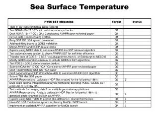
Objectives of the talk • Highlight the features of various “kf” Kalman filter geolocation models • Show how TrackIt works with sea-surface temperature matching • Help appreciate the details and practical usage of the “kf” models the wine tasting experience to geolocation
kftrack kfsst ukfsst Others e.g. tidal methods, Easy-Fish Tracker Manufacturer Software A common 2-step approach in geolocation • Get raw daily positions from tag manufacturer processing • Reconstruct most probable positions from the raw estimates • A disconnected one-way process – no feedback and limited use of the original time series • Extreme outliers are still problematic
Goals of the “kf” models To give us • a track of geographic positions • some ideas about the uncertainities • some quantitative movement parameters
The “kf” family Similarities • Underlying movement model • random walk with drift and diffusion • Observation model • predicts and describes observation error at any given position • Kalman filter (extended (EKF) or unscented (UKF) ) • Maximum likelihood estimated model parameters • Most probable track • Weighted average of what is learned from the current position’s data and the entire track Differences
Quick recap of the TrackIt model Nielsen & Sibert 2007. Can J Fish Aquat Sci 64 u, v – velocity in North-South, East-West direction D – diffusion
Raw geolocations vs. TrackIt Different scale
Drifter (with PAT attached) From M. Musyl (U Hawaii/ NOAA) 3 Mako sharks (SPOT+PAT) From S. Kohin and D. Holts (SWFSC) Data scenarios Low Sea-surface temperature (SST) imagery • Reynolds (NOAA old OI set) 1 deg, Weekly • NOAA OIsst version 1 (AVHRR only) 0.25 deg, Daily • Blended (D. Foley, Coastwatch) 0.1 deg, 5-day • MODIS Aqua (NASA GSFC) 0.05 deg, 8-day Light only vs. High Res
Usage tips Just give me the conclusions… • Always look at the confidence interval (ci) • SST may help, but not all the time • SST works best when there is a sharp gradient • Imagery resolution doesn’t matter too much • Pay attention to the smoothing radius (r) • Overall, SST reduces the width of the confidence region • Convergence for a fit is needed! Reduce the • No. of parameters estimated (e.g. bsst.ph = -1) • Resolution of SST imagery (e.g. Reynolds, fixed radius) Use • Better initial values (e.g. D.init = 300) … a balancing act
1. Swirl – General sense; Track segments are colored by month 2. Sip – Snip out segments, look at confidence interval (shaded) • 3. Taste – Understand SST, see how SST gradient matters Wine tasting guide to TrackIt What you will see + “True” positions (SPOT/GPS) Yellow line
A. B. C. D. Mako 1901
A. B. C. D. Mako 39322
A. B. C. D. Mako 1902
A. B. C. D. Drifter
Download http://www.soest.hawaii.edu/tag-data/software/ • R (2.8 and below) • NOT 2.9.0 (latest, released April, 2009) • A basic internal R function has changed for unzipping • Let us know when • it works! • it doesn’t… • You have • Double-tag data Chi Lam USC
Acknowledgements This work was sponsored by the Pelagic Fisheries Research Program, University of Hawaii. We thank Michael Musyl, Suzanne Kohin, David Holts, Dave Foley, Wildlife Computers, and Lotek Wireless for generously sharing data and ideas. NASA Earth System Science Fellowship Cheers!