Simplex Method
Simplex Method. MSci331 — Week 3~4. Simplex Algorithm. Consider the following LP, solve using Simplex:. Step 1: Preparing the LP. Step 2: Express the LP in a tableau form. Step 3: Obtain the initial basic feasible solution (if available). a) Set n - m variables equal to 0.

Simplex Method
E N D
Presentation Transcript
Simplex Method MSci331—Week 3~4
Simplex Algorithm • Consider the following LP, solve using Simplex:
Step 3: Obtain the initial basic feasible solution (if available) a) Set n-m variables equal to 0 These n-m variables the NBV b) Check if the remaining m variables satisfy the condition of BV = If yes, the initial feasible basic solution (bfs) is readily a available = else, carry on some ERO to obtain the initial bfs
Step 4: Apply the Simplex Algorithm a) Is the initial bfs optimal? (Will bringing a NBV improve the value of Z?) b) If yes, which variable from the set of NBV to bring into the set of BV? - The entering NBV defines the pivot column c) Which variable from the set of BV has to become NBV? - The exiting BV defines the pivot row Exits Pivot cell Enters
Summary of Simplex Algorithm for Papa Louis Set: n-m=0 m≠0 BFS (intial) BFS (1) BFS (2) BFS (3) 1 The optimal solution is x1=20, x2=60 The optimal value is Z=180 The BFS at optimality x1=20, x2=60, s3=20
Class activity • Consider the following LP: This is a maximizing LP, in normal form. So an initial BFS exists.
Class activity Make this coefficient equal 1 and pivot all other rows relative to it Exits Enters 4/1 6/1 2/2* ---
Class activity Make this coefficient equal 1 and pivot all other rows relative to it Enters 3/2.5* 5/3.5 --- 5/0.5
Example: LP model with Minimization Objective • Solve the following LP model: • Initial Tableau
Example: LP model with Minimization Objective • Iteration 0 • Iteration 1 • Optimality test:
> Constraint x2 40 35 30 25 20 15 10 5 5 10 15 20 25 30 35 40 Constraint 1 Constraint 3 Z Constraint 2 x1 Constraint 4 New feasible region
Equality Constraint x2 40 35 30 25 20 15 10 5 5 10 15 20 25 30 35 40 Constraint 1 Constraint 3 Z Constraint 2 x1 New feasible region
The Problem of Finding an Initial Feasible BV An LP Model Standard Form Cannot find an initial basic variable that is feasible.
Example: Solve Using the Big M Method Write in standard form
Example: Solve Using the Big M Method Adding artificial variables
Example: Solve Using the Big M Method Put in tableau form
Example: Solve Using the Big M Method Eliminating a2 from row 0 by operations: new Row 0 = old Row 0 -M*old Row 2
Example: Solve Using the Big M Method Eliminating a3 from the new row 0 by operations: new Row=old Row-M*old Row 3
Example: Solve Using the Big M Method The initial basic variables are s1=25, a2=12, and a3=0. Now ready to proceed for the simplex algorithm. The initial Tableau
Example: Solve Using the Big M Method Using EROs change the column of x1 into a unity vector. Iteration 1
Example: Solve Using the Big M Method Using EROs change the column of z into a unity vector. Iteration 2 Students to try more iterations. The solution is infeasible. See the attached solution.
Special case 1: Alternative Optima . See Notes on this slide (below) for more information
Special case 2: Unbounded LPs s1 0 1 x1 See Notes on this slide (below) for more information
Special Case 5: Degeneracy Iteration 0 Iteration 1 Iteration 2
Special Case 5: Degeneracy Degeneracy reveals from practical standpoint that the model has at least one redundant constraint.