Investigating Relationships between Variables: Interpreting Scatterplots
140 likes | 490 Vues
Investigating Relationships between Variables: Interpreting Scatterplots. Examining Relationships. Is there a relationship between the number of minutes the 1992 Dream Team basketball player was on the court and the number of points he scored?

Investigating Relationships between Variables: Interpreting Scatterplots
E N D
Presentation Transcript
Investigating Relationships between Variables:Interpreting Scatterplots
Examining Relationships • Is there a relationship between the number of minutes the 1992 Dream Team basketball player was on the court and the number of points he scored? • We can investigate this question by using techniques designed to look at the relationships among variables. • Although there are many of these, for now we will concentrate on those used to look at relationships between two quantitative variables
The 1992 “Dream Team” • In the 1992 Summer Olympics, the United States men’s basketball team, known as the Dream Team, won the gold medal. After winning all five preliminary games, they entered the single-elimination medal round along with seven other teams. The Dream Team then defeated Puerto Rico, Lithuania, and Croatia by an average score of 120 to 79 to claim the gold medal. The following table gives the cumulative box score for the United States players over these three final games.
Creating a Picture • Of course, we still want to follow the first rule of statistics---Draw a picture. • The plot we use to show relationships is called a scatterplot.
We think that the number of minutes a player is on the court will help to explain the number of points he scores, so “minutes” is our explanatory variable and is graphed along the horizontal or x-axis. • “Points” is our response variable, and is graphed along the vertical or y-axis.
Interpreting Scatterplots • When looking at the relationships between 2 quantitative variables, we want to consider any overall pattern that appears. • Three aspects help to guide our description: • Strength • Type (form) • Direction
Let’s start with strength--- • To help determine the strength of a relationship, think about drawing an oval around the data. Create, if you will, a “data cloud” • Interpretation: • A diagonal oval either increasing or decreasing indicates a relationship • The tighter the oval---the stronger the relationship • A horizontal oval indicates no relationship • A circle would indicate a weak or no relationship
The second element • Type (form)— • The type of relationship that exists can be described (at least for now) as either linear or nonlinear. • In other words, if we can summarize the data with a line (not a curve) through the middle of the data, we would consider the relationship to be linear. • If a curve would do a better job, then the relationship would be categorized as non-linear. (we’ll look at non-linear relationships later) We notice that a line, rather than a curve appears to summarize the data. (we’ll learn some additional ways to check this aspect later)
The last characteristic we use: • Direction: • To determine the direction of the relationship, we think about the how each variable is changing with respect to the other. • There are several ways to think about this. • A relationship is positive when above average values of one variable occur with above average values of the other variable. • We can also see the positive relationship in the scatterplot very quickly • As one variable is increasing, the other variable also increases
The scatterplot at the right shows horsepower ratings for several models of vehicles and the corresponding gas mileage. The scatterplot indicates that the relationship between these variables is negative • Again we can “see” the negative relationship between the variables in the scatterplot. • As one variable is increasing, the value of the second variable is decreasing. • A negative relationship occurs when above average values of one variable happen with below average values of the second variable.
Putting it all Together • Now that we know the individual elements for investigating the relationship between two quantitative variables, let’s see if we can summarize the association (another word for relationship) between the minutes on the court and the points scored for the 1992 Dream Team.
There appears to be a moderately strong* relationship between the number of minutes a player is on the court and the number of points he scored. As the time on court increases, so does the points scored, indicating a positive association between these variables. *Note: we will learn some numeric guidelines on strength in the next lesson about correlation.
Additional Resources • The Practice of Statistics: • 1st Edition: YMM—pg 106-111 • 2nd Edition: YMS—pg 120-140 • Against All Odds Video • Video #8---Describing Relationships