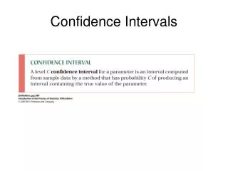
Confidence Intervals
Chapter 6. Confidence Intervals. Confidence Intervals for the Mean (Small Samples). § 6.2. The t - Distribution. When a sample size is less than 30, and the random variable x is approximately normally distributed, it follow a t - distribution. Properties of the t -distribution.

Confidence Intervals
E N D
Presentation Transcript
Chapter 6 Confidence Intervals
The t-Distribution When a sample size is less than 30, and the random variable x is approximately normally distributed, it follow a t-distribution. Properties of the t-distribution • The t-distribution is bell shaped and symmetric about the mean. • The t-distribution is a family of curves, each determined by a parameter called the degrees of freedom. The degrees of freedom are the number of free choices left after a sample statistic such as is calculated. When you use a t-distribution to estimate a population mean, the degrees of freedom are equal to one less than the sample size. • d.f. = n – 1 Degrees of freedom Continued.
d.f. = 2 d.f. = 5 t Standard normal curve 0 The t-Distribution • The total area under a t-curve is 1 or 100%. • The mean, median, and mode of the t-distribution are equal to zero. • As the degrees of freedom increase, the t-distribution approaches the normal distribution. After 30 d.f., the t-distribution is very close to the standard normal z-distribution. The tails in the t-distribution are “thicker” than those in the standard normal distribution.
Critical Values of t Example: Find the critical value tc for a 95% confidence when the sample size is 5. Appendix B: Table 5: t-Distribution d.f. = n – 1 = 5 – 1 = 4 tc = 2.776 c = 0.95 Continued.
c = 0.95 t tc = 2.776 tc = 2.776 Critical Values of t Example continued: Find the critical value tc for a 95% confidence when the sample size is 5. 95% of the area under the t-distribution curve with 4 degrees of freedom lies between t = ±2.776.
Confidence Intervals and t-Distributions Constructing a Confidence Interval for the Mean: t-Distribution In Words In Symbols • Identify the sample statistics n, , and s. • Identify the degrees of freedom, the level of confidence c, and the critical value tc. • Find the margin of error E. • Find the left and right endpoints and form the confidence interval. d.f. = n – 1 Left endpoint: ERight endpoint: +E Interval: E < μ< +E
Constructing a Confidence Interval Example: In a random sample of 20 customers at a local fast food restaurant, the mean waiting time to order is 95 seconds, and the standard deviation is 21 seconds. Assume the wait times are normally distributed and construct a 90% confidence interval for the mean wait time of all customers. n = 20 = 95 s = 21 d.f.= 19 tc = 1.729 86.9 < μ< 103.1 ± E = 95 ± 8.1 We are 90% confident that the mean wait time for all customers is between 86.9 and 103.1 seconds.
Use the normal distribution with If is unknown, use s instead. Yes Yes No No Yes Use the normal distribution with No Use the t-distribution with and n – 1 degrees of freedom. Normal or t-Distribution? Is n 30? Is the population normally, or approximately normally, distributed? You cannot use the normal distribution or the t-distribution. Is known?
Normal or t-Distribution? Example: Determine whether to use the normal distribution, the t-distribution, or neither. a.) n = 50, the distribution is skewed, s = 2.5 The normal distribution would be used because the sample size is 50. b.) n = 25, the distribution is skewed, s = 52.9 Neither distribution would be used because n < 30 and the distribution is skewed. c.) n = 25, the distribution is normal, = 4.12 The normal distribution would be used because although n < 30, the population standard deviation is known.


