Download
1 / 39
420 likes | 864 Vues
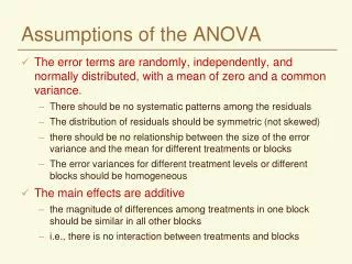
Assumptions of the ANOVA. The error terms are randomly, independently, and normally distributed, with a mean of zero and a common variance. There should be no systematic patterns among the residuals The distribution of residuals should be symmetric (not skewed)

E N D
Assumptions of the ANOVA • The error terms are randomly, independently, and normally distributed, with a mean of zero and a common variance. • There should be no systematic patterns among the residuals • The distribution of residuals should be symmetric (not skewed) • there should be no relationship between the size of the error variance and the mean for different treatments or blocks • The error variances for different treatment levels or different blocks should be homogeneous • The main effects are additive • the magnitude of differences among treatments in one block should be similar in all other blocks • i.e., there is no interaction between treatments and blocks
If the ANOVA assumptions are violated: • Affects sensitivity of the F test • Significance level of mean comparisons may be much different than they appear to be • Can lead to invalid conclusions
Diagnostics • Use descriptive statistics to test assumptions before you analyze the data • Means, medians and quartiles for each group (histograms, box plots) • Tests for normality, additivity • Compare variances for each group • Examine residuals after fitting the model in your analysis • Descriptive statistics of residuals • Normal plot of residuals • Plots of residuals in order of observation • Relationship between residuals and predicted values (fitted values)
SAS Box Plots • Look For • Outliers • Skewness • Common Variance • Caution • Not many observations per group
Additivity • Linear additive model for each experimental design Yij= + i + ij CRD Yij = + i + j+ ijRBD • Implies that a treatment effect is the same for all blocks and that the block effect is the same for all treatments
Water Table When the assumption would not be correct... • When there is an interaction between blocks and treatments - the model is no longer additive • may be multiplicative; for example, when one treatment always exceeds another by a certain percentage Two nitrogen treatments applied to 3 blocks 1 2 3 Differences between treatments might be greater in block 3
Testing Additivity --- Tukey’s test • Test is applicable to any two-way classification such as RBD classified by blocks and treatments • Compute a table with raw data, treatment means, treatment effects ( ), block meansand block effects ( ) Q = SYij ( ) ( ) • Compute SS for nonadditivity = (Q2*N)/(SST*SSB) with 1 df • The error term is partitioned into nonadditivity and residual and can be tested with F N = t*r Test can also be done with SAS
Residuals • Residuals are the error terms – what is left over after accounting for all of the effects in the model CRD RBD
Independence • Independence implies that the error (residual) for one observation is unrelated to the error for another • Adjacent plots are more similar than randomly scattered plots • So the best insurance is randomization • In some cases it may be better to throw out a randomization that could lead to biased estimates of treatment effects
Normality • Look at stem leaf plots, boxplots of residuals • Normal probability plots • Minor deviations from normality are not generally a problem for the ANOVA
Replicates Treatment 1 2 3 4 5 Total Mean s2 A 3 1 5 4 2 15 3 2.5 B 6 8 7 4 5 30 6 2.5 C 12 6 9 3 15 45 9 22.5 D 20 14 11 17 8 70 14 22.5 Homogeneity of Variances • Logic would tell us that differences required for significance would be greater for the two highly variable treatments
If we analyzed together: Source df SS MS F Treatments 3 330 110 8.8** Error 16 200 12.5 LSD=4.74 Analysis for A and B Source df SS MS F Treatments 1 22.5 22.5 9* Error 8 20.0 2.5 Conclusions would be different if we analyzed the two groups separately: Source df SS MS F Treatments 1 62.5 62.5 2.78 Error 8 180 22.5 Analysis for C and D
What the ANOVA assumes Independence of Means and Variances • A relationship between means and variances is the most common cause of heterogeneity of variance Test the effect of a new vitamin on the weights of animals. What you see
Examining the error terms • Take each observation and remove the general mean, the treatment effects and the block effects; what is left will be the error term for that observation The model = Block effect = Treatment effect = so ... then ... Finally ...
Looking at the error components Trt. I II III IV Mean A 47 52 62 51 53 B 50 54 67 57 57 C 57 53 69 57 59 D 54 65 74 59 63 Mean 52 56 68 56 58 Trt. I II III IV Mean A 0 1 -1 0 0 B -1 -1 0 2 0 C 4 -4 0 0 0 D -3 4 1 -2 0 Mean 0 0 0 0 0 e11 = 47 – 52 – 53 + 58 = 0
Looking at the error components Trt. I II III IV Mean A .18 .30 .28 .44 0.3 B .32 .4 .42 .46 0.4 C 2.0 3.0 1.8 2.8 2.4 D 2.5 3.3 2.5 3.3 2.9 E 108 140 135 165 137 F 127 153 148 176 151 Mean 40 50 48 58 49 Trt. I II III IV A 8.88 -1.00 0.98 -8.86 B 8.92 -1.00 1.02 -8.94 C 8.60 -0.40 0.40 -8.60 D 8.60 -0.60 0.60 -8.60 E -20.00 2.00 -1.00 19.00 F -15.00 1.00 2.00 16.00 e11 = 0.18 – 40 - 0.3 + 49 = 8.88
Residual Plots • A valuable tool for examining the validity of assumptions for ANOVA – should see a random scattering of points on the plot • For simple models, there may be a limited number of groups on the Predicted axis • Look for random dispersion of residuals
Residual Plots – Outlier Detection • Recheck data input • May have to treat as a missing plot if too extreme
Are the errors randomly distributed? • in this example the variance of the errors increases with the mean
Residual Plots • Errors are not independent • Model may not be adequate • e.g., fitting a straight regression line when response is curvilinear
Where t = number of independent variances (mean squares) that you are comparing v = degrees of freedom associated with each mean square Homogeneity Quick Test (F Max Test) • By examining the ratio of the largest variance to the smallest and comparing with a probability table of ratios, you can get a quick test. • The null hypothesis is that variances are equal, so if your computed ratio is greater than the table value (Kuehl, Table VIII), you reject the null hypothesis.
An Example An RBD experiment with four blocks to determine the effect of salinity on the application of N and P on sorghum 5437.99/9.03 = 602.21 Table value (t=7, v=r-1=3) = 72.9 602.21>72.9 Reject null hypothesis and conclude that variances are NOT homogeneous (equal)
Other HOV tests are more sensitive • If the quick test indicates that variances are not equal (homogeneous), no need to test further • But if quick test indicates that variances ARE homogeneous, you may want to go further with a Levene (Med) test or Bartlett’s test which are more sensitive. • This is especially true for values of t and v that are relatively small. • F max, Levene (Med), and Bartlett’s tests can be adapted to evaluate homogeneity of error variances from different sites in multilocational trials.
Homogeneity of Variances - Tests • Johnson (1981) compared 56 tests for homogeneity of variance and found the Levene (Med) test to be one of the best. • Based on deviations of observations from the median for each treatment group. Test statistic is compared to a critical F,t-1,N-t value. • This is now the default homogeneity of variance test in SAS (HOVTEST). • Bartlett’s test is also common • Based on a chi-square test with t-1 df • If calculated value is greater than tabular value, then variances are heterogeneous
What to do if assumptions are violated? • Divide your experiment into subsets of blocks or treatments that meet the assumptions and conduct separate analyses • Transform the data and repeat the analysis • residuals follow another distribution (e.g., binomial, Poisson) • there is a specific relationship between means and variances • residuals of transformed data must meet the ANOVA assumptions • Use a nonparametric test • no assumptions are made about the distribution of the residuals • most are based on ranks – some information is lost • generally less powerful than parametric tests • Use a Generalized Linear Model (PROC GLIMMIX in SAS) • make the model fit the data, rather than changing the data to fit the model
Independence between means and variances... • Can usually tell just by looking. Do the variances increase as the means increase? • If so, construct a table of ratios of variance to means and standard deviation to means • Determine which is more nearly proportional - the ratio that remains more constant will be the one more nearly proportional • This information is necessary to know which transformation to use – the idea is to convert a known probability distribution to a normal distribution
Comparing Ratios - Which Transformation? Trt Mean Var SDev Var/M SDev/M M-C 0.3 0.01147 0.107 0.04 0.36 M-V 0.4 0.00347 0.059 0.01 0.15 C-C 2.4 0.3467 0.589 0.14 0.24 C-V 2.9 0.2133 0.462 0.07 0.16 S-C 137.0 546.0 23.367 3.98 0.17 S-V 151.0 425.3 20.624 2.82 0.14 SDev roughly proportional to the means
The Log Transformation • When the standard deviations (not the variances) of samples are roughly proportional to the means, the log transformation is most effective • Common for counts that vary across a wide range of values • numbers of insects • number of diseased plants/plot • Also applicable if there is evidence of multiplicative rather than additive main effects • e.g., an insecticide reduces numbers of insects by 50%
General remarks... • Data with negative values cannot be transformed with logs • Zeros present a special problem • If negative values or zeros are present, add 1 to all data points before transforming • You can multiply all data points by a constant without violating any rules • Do this if any of the data points are less than 1 (to avoid negative logs)
Recheck... • After transformation, rerun the ANOVA on the transformed data • Recheck the transformed data against the assumptions for the ANOVA • Look at residual plots, normal plots • Carry out Levene’s test or Bartlett’s for homogeneity of variance • Apply Tukey’s test for additivity • Beware that a transformation that corrects one violation in assumptions may introduce another
Square Root Transformation • One of a family of power transformations • Use when you have counts of rare events in time or space • number of insects caught in a trap • The variance tends to be proportional to the mean • May follow a Poisson distribution • If there are counts under 10, it is best to use square root of Y + .5 • Will be easier to declare significant differences in mean separation • When reporting, “detransform” the means – present summary mean tables on original scale
Arcsin or Angular Transformation • Counts expressed as percentages or proportions of the total sample may require transformation • Follow a binomial distribution - variances tend to be small at both ends of the range of values ( close to 0 and 100%) • Not all percentage data are binomial in nature • e.g., grain protein is a continuous, quantitative variable that would tend to follow a normal distribution • If appropriate, it usually helps in mean separation
Arcsin or Angular Transformation • Data should be transformed if the range of percentages is greater than 40 • May not be necessary for percentages in the range of 30-70% • If percentages are in the range of 0-30% or 70-100%, a square root transformation may be better • Do not include treatments that are fixed at 0% or at 100% • Percentages are converted to an angle expressed in degrees or in radians • express Yij as a decimal fraction – gives results in radians • 1 radian = 57.296 degrees
Reasons for Transformation • We don’t use transformation just to give us results more to our liking • We transform data so that the analysis will be valid and the conclusions correct • Remember .... • all tests of significance and mean separation should be carried out on the transformed data • calculate means of the transformed data before “detransforming”