Download
1 / 26
280 likes | 498 Vues
L29: Sensitivity and Breakeven Analysis. ECON 320 Engineering Economics Mahmut Ali GOKCE Industrial Systems Engineering Computer Sciences. Chapter 10 Handling Project Uncertainty. Origin of Project Risk Methods of Describing Project Risk Probability Concepts for Investment Decisions

E N D
L29: Sensitivity and Breakeven Analysis ECON 320 Engineering Economics Mahmut Ali GOKCE Industrial Systems Engineering Computer Sciences
Chapter 10Handling Project Uncertainty • Origin of Project Risk • Methods of Describing Project Risk • Probability Concepts for Investment Decisions • Risk-Adjusted Discount Rate Approach
Origins of Project Risk • Risk: the potential for loss • Project Risk: variability in a project’s NPW • Risk Analysis: The assignment of probabilities to the various outcomes of an investment project
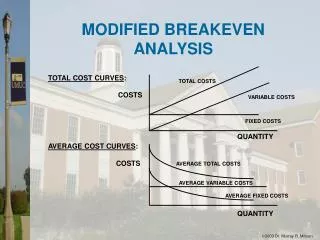
Methods of Describing Project Risk • Sensitivity Analysis: a means of identifying the project variables which, when varied, have the greatest effect on project acceptability. • What might have greatest effect on NPW, if changed? • Break-Even Analysis: a means of identifying the value of a particular project variable that causes the project to exactly break even. • Scenario Analysis: a means of comparing a “base case” to one or more additional scenarios, such as best and worst case, to identify the extreme and most likely project outcomes.
Sensitivity Analysis – Example 10.1Should we or should we not? • Transmission-Housing Project by Boston Metal Company • New investment = $125,000 • Number of units = 2,000 units • Unit Price = $50 per unit • Unit variable cost = $15 per unit • Fixed cost = $10,000/Yr • Project Life = 5 years • Salvage value = $40,000 at the end of project life. • Income tax rate = 40% • MARR = 15% • Depreciation 7-year MACRS (Check out % depreciation from table 8.5) for a 5 year project. • Develop a table for after-tax cash flow table! Then we will assess the situation under different scenarios
Example 10.1 - After-tax Cash Flow for BMC’s Transmission-Housings Project – “Base Case”
Example 10.2 - Sensitivity Analysis for Five Key Input Variables Try to understand what will happen if estimates on unit prices, demand, variable and fixed cost, salvage value change? Base
Sensitivity graph – BMC’s transmission-housings project $100,000 90,000 Unit Price 80,000 70,000 Demand 60,000 50,000 Salvage value 40,000 Fixed cost Base 30,000 Variable cost 20,000 10,000 0 -10,000 -15% -10% -5% -20% 0% 5% 10% 15% 20%
Example 10.2 - Sensitivity Analysis for Mutually Exclusive Alternatives
Capital (Ownership) Cost • Electrical power: CR(10%) = ($30,000 - $3,000)(A/P, 10%, 7) + (0.10)$3,000 = $5,845 • LPG: CR(10%) = ($21,000- $2,000)(A/P, 10%, 7) + (0.10)$2,000 = $4,103 • Gasoline: CR(10%) = ($20,000-$2,000)(A/P, 10%, 7) + (0.10) $2,000 = $3,897 • Diesel fuel: CR(10%) = ($25,000 -$2,200)(A/P, 10%, 7) +(0.10) $2,200 = $4,903
REMEMBER L 17 FROM CHAPTER 6 ? Annual Equivalent Cost • When only costs are involved, the AE method is called the annual equivalent cost. • Revenues must cover two kinds of costs: Operating costs and capital costs. Capital costs + Annual Equivalent Costs Operating costs
REMEMBER L 17 FROM CHAPTER 6 ?Capital (Ownership) Costs • Def: Owning an equipment is associated with two transactions—(1) its initial cost (I) and (2) its salvage value (S). • Capital costs: Taking these items into consideration, we calculate the capital costs as: S 0 N I 0 1 2 3 N CR(i)
Annual O&M Cost Let M be number of shifts per year • Electrical power: $500 + (1.60 + 5)M = $500 + 6.6M • LPG: $1,000 + (12 + 6)M = $1,000 + 18M • Gasoline: $800 + (13.2 + 7)M = $800 + 20.20M • Diesel fuel: $1,500 + (7.7 + 9)M = $1,500 + 16.7M
Annual Equivalent Cost • Electrical power: AE(10%) = 6,345 + 6.6M • LPG: AE(10%) = 5,103 + 18M • Gasoline: AE(10%) = 4,697 + 20.20M • Diesel fuel: AE(10%) = 6,403 + 16.7M
Break-Even Analysis • Excel using a Goal Seek function • Analytical Approach
NPW Breakeven Value Demand Excel Using a Goal Seek Function Can we find demand level for which NPW is 0?
Goal Seek Function Parameters
Analytical ApproachUnknown Sales Units (X) for BMC transm. housing
PW of cash inflows PW(15%)Inflow= (PW of after-tax net revenue) + (PW of net salvage value) + (PW of tax savings from depreciation = 30X(P/A, 15%, 5) + $37,389(P/F, 15%, 5) + $7,145(P/F, 15%,1) + $12,245(P/F, 15%, 2) + $8,745(P/F, 15%, 3) + $6,245(P/F, 15%, 4) + $2,230(P/F, 15%,5) = 30X(P/A, 15%, 5) + $44,490 = 100.5650X + $44,490
PW of cash outflows: PW(15%)Outflow = (PW of capital expenditure_ + (PW) of after-tax expenses = $125,000 + (9X+$6,000)(P/A, 15%, 5) = 30.1694X + $145,113 The NPW: PW (15%) = 100.5650X + $44,490 - (30.1694X + $145,113) =70.3956X - $100,623. Breakeven volume: PW (15%) = 70.3956X - $100,623 = 0 Xb =1,430 units.
$350,000 300,000 250,000 200,000 150,000 100,000 50,000 0 -50,000 -100,000 Inflow Break-even Volume Profit Outflow PW (15%) Xb = 1430 Loss 0 300 600 900 1200 1500 1800 2100 2400 Annual Sales Units (X) Break-Even Analysis Chart