Chapter 10 Sensitivity and Breakeven Analysis
Learn about project risks, sensitivity analysis, break-even analysis, and scenario analysis in investment decisions. Understand methods of describing project risk origins and analyzing uncertainties in cash flows.


Chapter 10 Sensitivity and Breakeven Analysis
E N D
Presentation Transcript
Handling Project Uncertainty • Origin of Project Risk • Methods of Describing Project Risk
Origins of Project Risk • Risk is to describe investment project where cash flows are not known in advance with certainty. Project risk on the other hand refer to variability in a project’s PW. In essence, we can see that risk is the potential for loss. • Risk Analysis is the assignment of probabilities to the various outcomes of an investment project.
Origins of Project Risk continue…. • The decision to make a major capital investment such as introducing a new product requires cash flow information over the life of a project. • The profitability estimate of an investment depends on cash flow estimations, which are generally uncertain. • The factors to be estimated include • the total market for the product; • the market share that the firm can attain; • the growth in the market; • the cost of producing the product, including labor and materials; • the selling price; • the life of a product; • the cost and the life of equipment needed; and • the effective tax rates. • Many of these factors are subject to uncertainty.
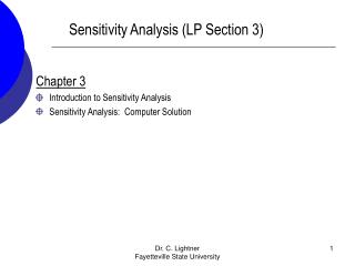
Methods of Describing Project Risk Fist, begin analyzing project risk by determining the uncertainty inbuilt in a project cash flows. We can do this analysis in a number of ways such as the following; Sensitivity Analysis (SA): Determines the effect on the PW of variations in the input variables (revenues, operating cost, and salvage value). SA is sometimes called “what if analysis” because it answers questions such as, • What if incremental sales are only 1,000 units, rather than 2,00 units? Then • what will be the NPW be?. • SA begins with a base-case situation, which is developed using most-likely values for each input. A useful way to present results of sensitivity analysis is to plot sensitivity graphs. Break-Even Analysis is a technique for studying the effect of variations in output on a firm’s NPW. Scenario Analysis is a technique that does consider the sensitivity of NPW to both changes in key variables and to the range of likely variable values. The decision maker may consider two extreme cases, a • “worst-case” scenario (low unit sales, high variable cost per unit, high fixed cost, and so on) and a • “best-case” scenario to identify the extreme and most likely project outcomes.
Sensitivity Analysis – Example 10.1 • Transmission-Housing Project by Boston Metal Company • New investment = $125,000 • Number of units = 2,000 units • Unit Price = $50 per unit • Unit variable cost = $15 per unit • Fixed cost = $10,000/Yr • Project Life = 5 years • Salvage value = $40,000 • Income tax rate = 40% • MARR = 15%
Example 10.1 - After-tax Cash Flow for BMC’s Transmission Housings Project – “Base Case”
Depreciation Calculation • Cost Base = $125,000 • Recovery Period = 7-year MACRS 8
Gains (Losses) associated with Asset Disposal • Salvage value = $40,000 • Book Value (year 5) = Cost Base – Total Depreciation • = $125,000 - $ 91,533 • = $ 33,467 • Taxable gains = Salvage Value – Book Value • = $40,000 - $ 33,467 • = $6,533 • Gains taxes = (Taxable Gains) (Tax Rate) • = $6,533 x (0.40) • = $2,613 9
Is this investment justifiable at a MARR of 15%? PW(15%) = -$125,000 + +$43,145(P/F, 15%, 1) + . . . . +$75,619(P/F, 15%, 5) = $40,169 > 0 Yes, Accept the Project $75,619 $48,245 $44,745 $42,245 $43,145 0 1 2 3 4 5 Years $125,000 12
Example 10.2 - Sensitivity Analysis for Five Key Input Variables Base
Sensitivity graph – BMC’s transmission-housings project (Example 10.2) $100,000 90,000 Unit Price 80,000 70,000 Demand 60,000 50,000 Salvage value 40,000 Fixed cost Base 30,000 Variable cost 20,000 10,000 0 -10,000 -15% -10% -5% -20% 0% 5% 10% 15% 20%
PW of cash inflows PW(15%)Inflow= (PW of after-tax net revenue) + (PW of net salvage value) + (PW of tax savings from depreciation = 30X(P/A, 15%, 5) + $37,389(P/F, 15%, 5) + $7,145(P/F, 15%,1) + $12,245(P/F, 15%, 2) + $8,745(P/F, 15%, 3) + $6,245(P/F, 15%, 4) + $2,230(P/F, 15%,5) = 30X(P/A, 15%, 5) + $44,490 = 100.5650X + $44,490
PW of cash outflows: PW(15%)Outflow = (PW of capital expenditure) + (PW) of after-tax expenses = $125,000 + (9X+$6,000)(P/A, 15%, 5) = 30.1694X + $145,113 The NPW: PW (15%) = 100.5650X + $44,490 - (30.1694X + $145,113) = 70.3956X - $100,623. Breakeven volume: PW (15%) = 70.3956X - $100,623 = 0 Xb = 1,430 units.
Break-Even Analysis Chart $350,000 300,000 250,000 200,000 150,000 100,000 50,000 0 -50,000 -100,000 Inflow Break-even Volume Profit Outflow PW (15%) Xb = 1430 Loss 0 300 600 900 1200 1500 1800 2100 2400 Annual Sales Units (X)