Faster algorithms for string matching problems: matching the convolution bound
Faster algorithms for string matching problems: matching the convolution bound. Piotr Indyk. 報告人 : 蕭志宣 田文錦 王弘倫. Outline. Introduction Randomized Boolean convolution Convolution over GF(2) in O(n)-time Application. Pattern matching. Input: two string t , p (text and patten)

Faster algorithms for string matching problems: matching the convolution bound
E N D
Presentation Transcript
Faster algorithms for string matching problems: matching the convolution bound Piotr Indyk 報告人: 蕭志宣 田文錦 王弘倫
Outline • Introduction • Randomized Boolean convolution • Convolution over GF(2) in O(n)-time • Application
Pattern matching • Input: two string t, p (text and patten) • Output: A binary sequence o o[i]=1 if p match t[i] o[i]=0 otherwise
Approach • Brute-force O(mn) time algorithm compares p with each of the string start at t(i), for i=1…n • A well-known algorithm KMP achieve O(m+n)
Fingerprint Approach • A fingerprint function Fp(Z)=Z mod p • Use F and compare F(p) and each of fingerprints F(t(j)) • The Monte Carlo algorithm for pattern matching requires O(n+m) time and has a probability of error O(1/n)
Use boolean convolution for string matching? • Solve application problem
1 1 0 0 0 0 0 0 1 1 1 1 1 1 1 1 1 1 0 0 1 1 1 1 1 1 1 0 0 1 1 0 Boolean convolution(,) 1 1 0 0 0 0 0 0 0 1 1 0 1 1 1 1 0 0 0 1 1 1 1
1 1 0 0 0 0 0 0 1 1 1 1 1 1 1 1 0 1 0 0 1 1 1 0 0 0 1 0 0 1 1 0 Polynomial convolution(+,)(over GF(2)) 1 1 0 0 0 0 0 0 0 1 1 0 1 1 1 1 0 0 0 1 1 0 0
a b a c c a c b a b a b a c b c a a a a 1 0 0 0 0 String matching VS. Boolean Convolution T Ta 1 0 1 0 0 1 0 0 1 0 1 0 1 0 0 P Oa Pa 1 0 1 0 1 1 1 0 0 1 1 0 0 1 0 1 Pa not
Boolean convolution u*v v 1 1 0 0 0 1 1 1 0 u Can be done in O(nlogn) o 1 1 0 0
Convolution on GF(2) u*v v 1 1 0 0 0 1 u 1 1 0 Can be done in O(n) 0 1 0 0 o’ Different from boolean convolution
Number of 1’s is…. • Odd output of convolution on GF(2) will be the same with boolean convolution • Even the position of 1 might be wrong…
o 1 1 0 0 Randomize? n bit Hamming space • Random choose r from Hn uniformly and conjunct r and u ru Correct boolean convolution output u 1 1 0 v 1 1 0 0 0 1 ru 0 1 0 r 0 1 0 ru 0 1 0 1 0 0 0 o’ Output wrong 0 Output correct 1
Lemma 1 • If(u*v)[i]=0 then o’[i]=0 • If(u*v)[i]=1 then Pr[o’[i]=1]=1/2
Expected error probability of position i after executer d times • o[i]=1 if o’[i]=1 in outcome of one execution • o[i]=0 with error probability of 1/2d
Error probability of convolution • Worst case All position output wrong 0 1/2d per position Probability of outputing a wrong convolution is O(n/2d)
Outline • Introduction • Randomized Boolean convolution • Convolution over GF(2) in O(n)-time • Application
Naturally… • Convolution is like the multiplication of two polynomial. • Therefore, the time complexity of FFT (Fast Fourier Transform) O(nlogn) is an upper bound of convolution.
GF(2) vs. GF(2t) • An element of GF(2t) can be defined as a polynomial of degree less than t over GF(2). • The operation of two elements over GF(2t) corresponds to the operation of two polynomials over GF(2). • e.g.- a, b GF(2t), ab over GF(2t) corresponds to a(x)b(x) mod u(x) over GF(2), (u(x) is an irreducible polynomial).
O(n)-time algorithm for polynomial multiplication over GF(2) • Step1: Reduce multiplication of p and q to a multiplication of two polynomials p’ and q’ of degree n/t over GF(2t), such that n/t= 2t, for t = O(logn). • Step2: Multiply p’ and q’ over GF(2t).
n=8, t=2 Elements in GF(2) 1 0 0 1 0 1 1 1 1 0 0 1 0 1 1 1 Elements in GF(22)
Step2 • Using O( log ) operations. • Thus we only need to show each operation can be done in O(1) time. • We can view a coefficients over GF(2t) as a polynomial over GF(2). • Therefore, we need to consider addition, multiplication, and modulus of polynomials of degree t over GF(2).
Addition over GF(2t) • Constant time since each element is of size O(logn), thus the addition can be performed in constant time (RAM model).
The more we need to know • Compute the product d(x) of polynomials a(x) and b(x). • Compute d(x) mod u(x), where u(x) is an irreducible polynomial of degree t (which can be found in negligible time during preprocessing)
Main idea • Shift the polynomial u by t/c (instead of 1) position. • There are only c necessary steps. • For each step, we use a lookup table and thus each operation can in constant time.
Multiplication • By FFT, each multiplication can be done in O( log ). • There are (2 )2 possible products. • Thus, we need (2 )2O( log ) = ( ) O( log ) = O(n) to build the lookup table.
Illustration t/c t/c … t/c t/c t/c … t/c
Division • Naturally, we have an O(t) algorithm (for d(x) & u(x) of degree 2t & t, respectively). • For i = 2t-1…t • Step1: check if the ith coefficient of di is 1. • Step2: if so , assign di-1 = di– u; otherwise set di-1 = di.
Illustration Each si has length t/c • d(x) = u(x)s(x)+ k(x) = u(x)(s1(x)+s2(x)+…+sc(x))+k(x) d(x) – u(x)s1(x) = u(x)(s2(x)+…+sc(x))+k(x) … we can compute k(x) after c steps. Constant time Constant time
Lookup table • Each component needs t/c time. • There are O(2t/c) elements (since u is unique, and d has length t/c). • t/c 2t/c ≤ t/c 2t =t/c n/t = O(n). • Thus, we need O(n) time to build the table.
So far… • We have a O(n) algorithm to multiply two polynomials of degree n over GF(2). • In other semiring, a convolution still needs O(nlogn) time.
Outline • Introduction • Randomized Boolean convolution • Convolution over GF(2) in O(n)-time • Application
String matching with don’t cares T A A D C C G E D A A C D E A C A B A A A * C C P A A D * C * = don’t cares
a b a c c a c b a b a b a c b c a a a a 1 0 0 0 0 String matching VS. Boolean Convolution T Ta 1 0 1 0 0 1 0 0 1 0 1 0 1 0 0 P Oa Pa 1 0 1 0 1 1 1 0 0 1 1 0 0 1 0 1 Pa not
T a b * a * b b c P a * b Example a = 101 b = 100 c = 010 * = 000 t1 0 0 0 0 0 0 0 1 t2 1 1 0 1 0 1 1 0 t3 0 1 0 0 0 1 1 1 a1 0 0 0 0 0 1 a2 0 0 0 0 0 0 p1 1 0 1 a3 0 1 0 0 0 1 p2 0 0 0 p3 1 0 0 a 0 1 0 0 0 1 anot 1 0 1 1 1 0
Analysis(1/2) • Lemma 2For any α>0 there is a constant c>0 such that the occurrence vector generated by the algorithm is correct with probability 1-1/nα Proof: Case 1. if p occurs in t at position i, then aj[i] = 0 with probability 1 for any j = 0…d-1 a * a * * a a *
Analysis(2/2) a = 101 b = 100 c = 010 * = 000 1 0 1 a bnot 0 1 1
Time Complexity O(n) O(log n)
Subset Matching • Input: A set-string T and a set-string P . • Output: All occurrences of P in T. a b c a c b c a c c e f b f b T = a c c b P =
Tree Pattern Matching and Subset Matching in Randomized O(nlog3m) Time, Proc.STOC’97,1997 R.Cole, R. Hariharan Give a very elegant O(nlog2n)-time randomized algorithm for this problem. We can replace the exact computation of boolean convolution by the probabilistic one. => time complexity O(nlogn)

