Chapter 8 Switching
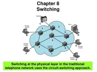
Chapter 8 Switching. Switching at the physical layer in the traditional telephone network uses the circuit-switching approach. Figure 8.1 Switched network. Figure 8.2 Taxonomy of switched networks. CIRCUIT-SWITCHED NETWORKS.

Chapter 8 Switching
E N D
Presentation Transcript
Chapter 8 Switching Switching at the physical layer in the traditional telephone network uses the circuit-switching approach.
Figure 8.1 Switched network Figure 8.2 Taxonomy of switched networks
CIRCUIT-SWITCHED NETWORKS • A circuit-switched network consists of a set of switches connected by physical links. A connection between two stations is a dedicated path made of one or more links. However, each connection uses only one dedicated channel on each link. Each link is normally divided into n channels by using FDM or TDM. • has three phases • Establish • Transfer • Disconnect • inefficient • channel capacity dedicated for duration of connection • if no data, capacity wasted • set up (connection) takes time • once connected, transfer is transparent
Figure 8.3 A trivial circuit-switched network A circuit-switched network is made of a set of switches connected by physical links, in which each link is divided into n channels.
Public Circuit Switched Network Circuit Establishment
Packet Switching In a packet-switched network, there is no resource reservation; resources are allocated on demand. • circuit switching was designed for voice • packet switching was designed for data • transmitted in small packets • packets contains user data and control info • user data may be part of a larger message • control info includes routing (addressing) info • packets are received, stored briefly (buffered) and past on to the next node
Packet Switching Datagram Approach Packet Switching Virtual Circuit Approach
Blocking or Non-blocking • blocking network • may be unable to connect stations because all paths are in use • used on voice systems • non-blocking network • permits all stations to connect at once • used for some data connections
8-4 STRUCTURE OF A SWITCH Figure 8.17 Crossbar switch with three inputs and four outputs
Figure 8.18 Multistage switch In a three-stage switch, the total number of crosspoints is 2kN + k(N/n)2 which is much smaller than the number of crosspoints in a single-stage switch (N2).
Example 8.3 Design a three-stage, 200 × 200 switch (N = 200) with k = 4 and n = 20. Solution In the first stage we have N/n or 10 crossbars, each of size 20 × 4. In the second stage, we have 4 crossbars, each of size 10 × 10. In the third stage, we have 10 crossbars, each of size 4 × 20. The total number of crosspoints is 2kN + k(N/n)2, or 2000 crosspoints. This is 5 percent of the number of crosspoints in a single-stage switch (200 × 200 = 40,000). According to the Clos criterion: n = (N/2)1/2 k > 2n – 1 Crosspoints ≥ 4N [(2N)1/2 – 1]
Example 8.4 Redesign the previous three-stage, 200 × 200 switch, using the Clos criteria with a minimum number of crosspoints. Solution We let n = (200/2)1/2, or n = 10. We calculate k = 2n − 1 = 19. In the first stage, we have 200/10, or 20, crossbars, each with 10 × 19 crosspoints. In the second stage, we have 19 crossbars, each with 10 × 10 crosspoints. In the third stage, we have 20 crossbars each with 19 × 10 crosspoints. The total number of crosspoints is 20(10 × 19) + 19(10 × 10) + 20(19 ×10) = 9500.
Figure 8.19 Time-slot interchange Time Division Switching • modern digital systems use intelligent control of space & time division elements • use digital time division techniques to set up and maintain virtual circuits • partition low speed bit stream into pieces that share higher speed stream • individual pieces manipulated by control logic to flow from input to output
Figure 8.22 Input port Figure 8.23 Output port
In Channel Signaling • Use same channel for signaling and call • Requires no additional transmission facilities • Inband • Uses same frequencies as voice signal • Can go anywhere a voice signal can • Impossible to set up a call on a faulty speech path • Out of band • Voice signals do not use full 4kHz bandwidth • Narrow signal band within 4kHz used for control • Can be sent whether or not voice signals are present • Need extra electronics • Slower signal rate (narrow bandwidth)
Drawbacks of In Channel Signaling • Limited transfer rate • Delay between entering address (dialing) and connection • Overcome by use of common channel signaling
Common Channel Signaling • Control signals carried over paths independent of voice channel • One control signal channel can carry signals for a number of subscriber channels • Common control channel for these subscriber lines • Associated Mode • Common channel closely tracks interswitch trunks • Disassociated Mode • Additional nodes (signal transfer points) • Effectively two separate networks