Chapter 2 Probability
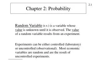
PROBABILITY (6MTCOAE205 ). Chapter 2 Probability. Important Terms. Random Experiment – a process leading to an uncertain outcome Basic Outcome – a possible outcome of a random experiment Sample Space – the collection of all possible outcomes of a random experiment

Chapter 2 Probability
E N D
Presentation Transcript
PROBABILITY (6MTCOAE205) Chapter 2 Probability
Important Terms • Random Experiment – a process leading to an uncertain outcome • Basic Outcome – a possible outcome of a random experiment • Sample Space – the collection of all possible outcomes of a random experiment • Event – any subset of basic outcomes from the sample space
Important Terms (continued) • Intersection of Events – If A and B are two events in a sample space S, then the intersection, A ∩ B, is the set of all outcomes in S that belong to both A and B S A AB B
Important Terms (continued) • A and B are Mutually Exclusive Events if they have no basic outcomes in common • i.e., the set A ∩ B is empty S A B
Important Terms (continued) • Union of Events – If A and B are two events in a sample space S, then the union, A U B, is the set of all outcomes in S that belong to either A or B S The entire shaded area represents A U B A B
Important Terms (continued) • Events E1, E2, … Ek are Collectively Exhaustive events if E1U E2U . . . U Ek = S • i.e., the events completely cover the sample space • The Complement of an event A is the set of all basic outcomes in the sample space that do not belong to A. The complement is denoted S A
Examples Let the Sample Space be the collection of all possible outcomes of rolling one die: S = [1, 2, 3, 4, 5, 6] Let A be the event “Number rolled is even” Let B be the event “Number rolled is at least 4” Then A = [2, 4, 6] and B = [4, 5, 6]
Examples (continued) S = [1, 2, 3, 4, 5, 6] A = [2, 4, 6] B = [4, 5, 6] Complements: Intersections: Unions:
Examples (continued) • Mutually exclusive: • A and B are not mutually exclusive • The outcomes 4 and 6 are common to both • Collectively exhaustive: • A and B are not collectively exhaustive • A U B does not contain 1 or 3 S = [1, 2, 3, 4, 5, 6] A = [2, 4, 6] B = [4, 5, 6]
Probability 3.2 • Probability – the chance that an uncertain event will occur (always between 0 and 1) 1 Certain .5 0 ≤ P(A) ≤ 1 For any event A 0 Impossible
Assessing Probability • There are three approaches to assessing the probability of an uncertain event: 1. classical probability • Assumes all outcomes in the sample space are equally likely to occur
Counting the Possible Outcomes • Use the Combinations formula to determine the number of combinations of n things taken k at a time • where • n! = n(n-1)(n-2)…(1) • 0! = 1 by definition
Assessing Probability Three approaches (continued) 2. relative frequency probability • the limit of the proportion of times that an event A occurs in a large number of trials, n 3.subjective probability an individual opinion or belief about the probability of occurrence
Probability Postulates 1. If A is any event in the sample space S, then 2. Let A be an event in S, and let Oi denote the basic outcomes. Then (the notation means that the summation is over all the basic outcomes in A) 3. P(S) = 1
Probability Rules 3.3 • The Complement rule: • The Addition rule: • The probability of the union of two events is
A Probability Table Probabilities and joint probabilities for two events A and B are summarized in this table:
Addition Rule Example Consider a standard deck of 52 cards, with four suits: ♥ ♣ ♦ ♠ Let event A = card is an Ace Let event B = card is from a red suit
Addition Rule Example (continued) P(Red UAce) = P(Red) + P(Ace) - P(Red∩Ace) = 26/52 + 4/52 - 2/52 = 28/52 Don’t count the two red aces twice! Color Type Total Red Black 2 2 4 Ace 24 24 48 Non-Ace 26 26 52 Total
Conditional Probability • A conditional probability is the probability of one event, given that another event has occurred: The conditional probability of A given that B has occurred The conditional probability of B given that A has occurred
Conditional Probability Example • What is the probability that a car has a CD player, given that it has AC ? i.e., we want to find P(CD | AC) • Of the cars on a used car lot, 70% have air conditioning (AC) and 40% have a CD player (CD). 20% of the cars have both.
Conditional Probability Example (continued) • Of the cars on a used car lot, 70% have air conditioning (AC) and 40% have a CD player (CD). 20% of the cars have both. CD No CD Total .2 .5 .7 AC .2 .1 No AC .3 .4 .6 1.0 Total
Conditional Probability Example (continued) • Given AC, we only consider the top row (70% of the cars). Of these, 20% have a CD player. 20% of 70% is 28.57%. CD No CD Total .2 .5 .7 AC .2 .1 No AC .3 .4 .6 1.0 Total
Multiplication Rule • Multiplication rule for two events A and B: • also
Multiplication Rule Example P(Red ∩Ace) = P(Red| Ace)P(Ace) Color Type Total Red Black 2 2 4 Ace 24 24 48 Non-Ace 26 26 52 Total
Statistical Independence • Two events are statistically independent if and only if: • Events A and B are independent when the probability of one event is not affected by the other event • If A and B are independent, then if P(B)>0 if P(A)>0
Statistical Independence Example • Of the cars on a used car lot, 70% have air conditioning (AC) and 40% have a CD player (CD). 20% of the cars have both. • Are the events AC and CD statistically independent? CD No CD Total .2 .5 .7 AC .2 .1 No AC .3 .4 .6 1.0 Total
Statistical Independence Example (continued) CD No CD Total .2 .5 .7 AC .2 .1 No AC .3 .4 .6 1.0 Total P(AC ∩ CD) = 0.2 P(AC) = 0.7 P(CD) = 0.4 P(AC)P(CD) = (0.7)(0.4) = 0.28 P(AC ∩ CD) = 0.2 ≠ P(AC)P(CD) = 0.28 So the two events are not statistically independent
Bivariate Probabilities 3.4 Outcomes for bivariate events:
Joint and Marginal Probabilities • The probability of a joint event, A ∩ B: • Computing a marginal probability: • Where B1, B2, …, Bk are k mutually exclusive and collectively exhaustive events
Marginal Probability Example P(Ace) Color Type Total Red Black 2 2 4 Ace 24 24 48 Non-Ace 26 26 52 Total
Using a Tree Diagram P(AC ∩ CD) = .2 Given AC or no AC: Has CD P(AC)= .7 Does not have CD P(AC ∩ CD) = .5 Has AC All Cars Does not have AC P(AC ∩ CD) = .2 Has CD P(AC)= .3 Does not have CD P(AC ∩ CD) = .1
Odds • The odds in favor of a particular event are given by the ratio of the probability of the event divided by the probability of its complement • The odds in favor of A are
Odds: Example • Calculate the probability of winning if the odds of winning are 3 to 1: • Now multiply both sides by 1 – P(A) and solve for P(A): 3 x (1- P(A)) = P(A) 3 – 3P(A) = P(A) 3 = 4P(A) P(A) = 0.75
Overinvolvement Ratio • The probability of event A1 conditional on event B1 divided by the probability of A1 conditional on activity B2 is defined as the overinvolvement ratio: • An overinvolvement ratio greater than 1 implies that event A1 increases the conditional odds ration in favor of B1:
Bayes’ Theorem 3.5 • where: Ei = ith event of k mutually exclusive and collectively exhaustive events A = new event that might impact P(Ei)
Bayes’ Theorem Example • A drilling company has estimated a 40% chance of striking oil for their new well. • A detailed test has been scheduled for more information. Historically, 60% of successful wells have had detailed tests, and 20% of unsuccessful wells have had detailed tests. • Given that this well has been scheduled for a detailed test, what is the probability that the well will be successful?
Bayes’ Theorem Example (continued) • Let S = successful well U = unsuccessful well • P(S) = .4 , P(U) = .6 (prior probabilities) • Define the detailed test event as D • Conditional probabilities: P(D|S) = .6 P(D|U) = .2 • Goal is to find P(S|D)
Bayes’ Theorem Example (continued) Apply Bayes’ Theorem: So the revised probability of success (from the original estimate of .4), given that this well has been scheduled for a detailed test, is .667