Chapter 1 Introduction

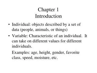
Chapter 1Introduction • Individual: objects described by a set of data (people, animals, or things) • Variable: Characteristic of an individual. It can take on different values for different individuals. Examples: age, height, gender, favorite class, speed, moisture, etc.

Types of Variables • Quantitative: numerical values, can be added, subtracted, averaged, etc. • ________: takes on values which are spaced. That is, for two values of a discrete variable that are adjacent, there is no value that goes between them. • ________: values are all numbers in a given interval. That is, for two values of a continuous variable that are adjacent, there is another value that can go between the two. • Categorical: An individual is placed into one of several groups or categories. These groups or categories are not usually numerical.

Types of Variables Examples: Numeric Variable Discrete Continuous Categorical Length Hours Enrolled Major Zip Code

Distribution of a Variable • The distribution of a variable tells us the possible values for the variable and the probability that the variable takes these values. • Two ways to describe a distribution • Numerically • Graphically

Categorical Variables • Suppose we poll 46 people on an issue. How can we exhibit their response? • Numerically: • Counts • Proportions • Percentages • Graphically: • Frequency Tables • Bar Charts • Pie Charts

Categorical Variables • Suppose we poll 46 people on an issue. How can we exhibit their response? • Frequency Tables: • counts (14 agree) • proportions (14/46 = .304 agree) • percents (30.4% agree)

Categorical Variables • Suppose we poll 46 people on an issue. How can we exhibit their response? • Bar Chart: can have counts, percents or proportions on vertical axis

Categorical Variables • Suppose we poll 46 people on an issue. How can we exhibit their response? • Pie Chart:

Examining a Distribution • To describe a distribution we need 3 items: • Shape: modes, symmetric, skewed • Center: mean, median • Spread: range, standard deviation, IQR • Look for the overall pattern and for striking deviations • Outlier-individual value that falls outside the overall pattern

Numeric Variable Distributions Shape: Modes: Major peaks in the distribution Symmetric: The values smaller and larger than the midpoint are mirror images of each other Skewed to the right: Right tail is much longer than the left tail Skewed to the left: Left tail is much longer than the right tail Center: Mean: The arithmetic average. Add up the numbers and divide by the number of observations. Median: List the data from smallest to largest. If there are an odd number of data values, the median is the middle one in the list. If there are an even number of data values, average the middle two in the list

Numeric Variable Distributions Spread: Range: The difference in the largest and smallest value. (Max – Min) Standard Deviation: Measures spread by looking at how far observations are from their mean. The computational formula for the standard deviation is Interquartile Range (IQR): Distance between the first quartile (Q1) and the third quartile (Q3). IQR = Q3– Q1 Q1 – 25% of the observations are less than Q1 and 75% are greater than Q1. Q3 – 75% of the observations are less than Q3 and 25% are greater than Q3.

Numeric Variable Distributions • Example 1.5 on page 11 of the book shows how much 50 consecutive shoppers spent in a store. The data appear as follows:

Numerical Variables • How can we describe the distribution of these 50 numbers? • Numerically • Center: Mean or Median • Spread: Quartiles, Range, IQR, or Standard deviation • Graphically • Frequency Table • Histogram • Boxplot • Stem and Leaf • Normal Quantile Plot

Descriptive statistics The descriptives box from SPSS gives the mean, median, variance, standard deviation, minimum, maximum, range, and IQR.

Percentiles • 50th percentile is also called the median – the middle data value if ordered smallest to largest • 25th and 75th percentiles are also called the quartiles: Q1 and Q3 respectively – the middle data value of each half

Frequency Table • Notice the amount spent is broken into categories or groups • Recall, frequency tables can be used for categorical variables as well

Histogram • Breaks the range of values of a variable into intervals (midpoint is displayed here) • Displays only the count or percent of the observations that fall into each interval

Box Plot Minimum, Q1, Median, Q3, and Maximum These five numbers are called the ____________________ What are these points?

Stem and Leaf Plot • Works best for smaller data sets • Example 1.4 on pg 10 • Here are the numbers of homeruns that Babe Ruth hit in each of his 15 years with the New York Yankees from 1920-1934: • 54, 59, 35, 41, 46, 25, 47, 60, 54, 46, 49, 46, 41, 34, 22

Normal Quantile Plot • Normal Quantile Plot (This compares the distribution of the sample to the Normal Distribution): the straight line is normal, compare dots to the line If dots fall close to the normal line then the data comes from a normal distribution.

Describing Numeric Variable Distributions • Now, we examine the appearance of other data: • Modes are major peaks in the distribution The histogram below The histogram below has one has two modes-bimodal mode-unimodal

Describing Numeric Variable Distributions • Now, we examine the appearance of other data: • This example is called right This is an example of a boxplot skewed since the distribution has that is skewed to the _______. a long right tail.

Describing Numeric Variable Distributions • ________: observations that are unusually far from the bulk of the data. • What are some possible explanations for outliers? • The data point was recorded wrong. • The data point wasn’t actually a member of the population we were trying to sample. • We just happened to get an extreme value in our sample. • The 1.5 x IQR Criterion for Outliers: Designate an observation a suspected outlier if it falls more than 1.5 x IQR below the first quartile or above the third quartile.

1.5*IQR Criterion Example • Suppose you had the following data set: -2, 15, 3, 7, 10, 21, 1, 5, 12, 8, 1, 35, 10 List data from smallest to largest: Find Q1, Median, Q3, Min, and Max: IQR = Q3 – Q1 = ______ 1.5*IQR = _______ Q1 – 1.5*IQR = ________If less than this number, then outlier Q3 + 1.5*IQR = ________If more than this number, then outlier Are there any outliers in this data set?

Describing Numeric Variable Distributions • Symmetry versus Skewness: __________ _________ ___________

Mean versus Median: • For a skewed distribution, the mean is farther out in the longer tail than is the median. mean<median mean=median mean>median To describe distributions use: Median and IQR Mean and standard deviation Median and IQR Symmetric Right Skewed Left Skewed

Strategy for Exploring Data on a Single Quantitative Variable • Always plot your data: make a graph usually a stem and leaf or histogram • Look for overall pattern and for outliers • Calculate an appropriate numerical summary to briefly describe center and spread • Sometimes the overall pattern of a large number of observations is so regular that it can be described by a smooth curve

Introducing the Normal Distribution It is customary to describe a normal distribution in the following way: Properties of the Normal Distribution: • Symmetric, bell-shaped • Mean, μ and standard deviation, σ • Area under the curve is 1 s m

The Normal Distribution Normal distributions can take on many different means and standard deviations. Only the general bell shape must remain the same. Here are some examples of normal distributions: m = -2 m = 0 m = 3 s = 0.5 s = 1 s = 2 -2 0 3

Distribution Properties • Introducing: The Standard Normal Distribution Properties: 1. _________________ 2. _________________ 3. _________________

Distribution Properties • Empirical Rule (The 68-95-99.7 Rule): If the distribution is normal, then • Approximately 68% of the data falls within one standard deviation of the mean • Approximately 95% of the data falls within two standard deviations of the mean • Approximately 99.7% of the data falls within three standard deviations of the mean

Distribution PropertiesEmpirical Rule

Percentiles of a Standard Normal Curve

Empirical Rule Example • If the grades on an exam are normally distributed with a mean of 68 and a variance of 16, what grade do you have to make to be in the top 15% of the class?

Distribution Properties • Shift Changes: adding or subtracting a number from the each of the values. mean mean + c mean - c

Distribution Properties • The mean, median, Q1, Q3, minimum, and maximum all shift when there is a shift change. The shift change, say c, is added or subtracted to each of the statistics accordingly. • The measures of spread (standard deviation, variance, IQR, and range) do not change when there is a shift change.

Distribution Properties • Scale Changes: multiplying or dividing each of the values by a number. mean

Distribution Properties • Scale Changes: multiplying or dividing each of the values by a number. mean*c

Distribution Properties • Scale Changes: multiplying or dividing each of the values by a number. mean/c

Distribution Properties • The mean, median, Q1, Q3, minimum, and maximum all change when there is a scale change unless they are zero. Each is multiplied or divided by the scale change c. • The measures of spread (standard deviation, variance, IQR, and range) always change when there is a scale change. The standard deviation, IQR, and range are multiplied or divided by the scale change c. The variance is multiplied or divided by c2.

Shift Change Example • Suppose we measure the weight of everyone on a football team and obtain the following statistics for a team report: • Mean: 230 lbs. Median: 240 lbs. • Std. Dev.: 50 lbs. Q1: 200 lbs., Q3: 280 lbs. • Variance: 2500 sq. lbs. IQR: 80 lbs • Min.: 170 lbs. Range: 180 lbs. • Max.: 350 lbs.

Shift Change Example • Now suppose we found out the scale was 10 lbs. under so we need to add 10 lbs. to every weight. What would happen to each of the following statistics? Original After Shift Change • Mean: 230 lbs. Mean:________ • Median: 240 lbs. Median:_________ • s: 50 lbs. s:_______ • Q1: 200 lbs. Q1:________ • Q3: 280 lbs. Q3:________

Shift Change Example • Now suppose we found out the scale was 10 lbs. under so we need to add 10 lbs. to every weight. What would happen to each of the following statistics? Original After Shift Change • Variance: 2500 sq. lbs. • Variance: ________ • IQR: 80 lbs. • IQR: _________ • Min: 170 lbs. • Min: _________ • Max: 350 lbs. • Max: _________ • Range: 180 lbs. • Range: _________

Shift and Scale Change Example • Further, suppose we found out that we are supposed to report the weights and statistics in kilograms, not lbs (Remember, 1 lb = 0.6 kilograms). What would happen to each of the following statistics? After Shift Change After Shift and Scale Change • Mean: 240 lbs. • Mean: ______________ • Median: 250 lbs. • Median: ______________ • s: 50 lbs. • s: _____________ • Q1: 210 lbs. • Q1: _____________ • Q3: 290 lbs. • Q3: _____________

Shift and Scale Change Example • Further, suppose we found out that we are supposed to report the weights and statistics in kilograms, not lbs (Remember, 1 lb = 0.6 kilograms). What would happen to each of the following statistics? After Shift Change After Shift and Scale Change • Variance: 2500 sq. lbs. • Variance: _______________ • IQR: 80 lbs. • IQR: _______________ • Min: 180 lbs. • Min: _______________ • Max: 360 lbs. • Max: ________________ • Range: 180 lbs. • Range: _________________

Linear Transformations • If you are given a mean, (or ), and a standard deviation, s (or ), and want to convert your data so you have a new mean, (or new), and new standard deviation, snew (or new), all you need is to remember what shift and scales changes affect. • In our linear transformation formula: • a is the shift change • b is the scale change • Standard deviation are only affected by scale changes, but means are affected by both shift and scales changes.

Linear Transformation Example • For example: = 12 and s = 7 but we want = 25 and = 10. snew = scale*s 10 = scale*7 scale = 10/7 scale = 1.43 • substituting in: = shift + scale* 25 = shift + 1.43*12 shift = 25  1.43*12 shift = 7.84 • So our linear transformation equation is: x new = 7.84 + 1.43*x

Chapter 1 Introduction