Part 2: part-based models

1. Part 2: part-based models by Rob Fergus (MIT)

2. Problem with bag-of-words • All have equal probability for bag-of-words methods • Location information is important

3. Overview of section • Representation • Computational complexity • Design choices • Recognition • Learning • Automated methods

4. Representation

5. Model: Parts and Structure

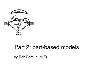
6. Representation • Object as set of parts • Generative representation • Model: • Relative locations between parts • Appearance of part • Issues: • How to model location • How to represent appearance • Sparse or dense (pixels or regions) • How to handle occlusion/clutter Figure from [Fischler73]

7. Example scheme • Model shape using Gaussian distribution on location between parts • Model appearance as pixel templates • Represent image as collection of regions • Extracted by template matching: normalized-cross correlation • Manually trained model • Click on training images

8. Sparse representation • + Computationally tractable (105 pixels  101 -- 102 parts) • + Generative representation of class • + Avoid modeling global variability • + Success in specific object recognition • - Throw away most image information • - Parts need to be distinctive to separate from other classes

9. History of Idea • Fischler & Elschlager 1973 • Yuille ‘91 • Brunelli & Poggio ‘93 • Lades, v.d. Malsburg et al. ‘93 • Cootes, Lanitis, Taylor et al. ‘95 • Amit & Geman ‘95, ‘99 • Perona et al. ‘95, ‘96, ’98, ’00 • Felzenszwalb & Huttenlocher ’00 • Many papers since 2000

10. The correspondence problem • Model with P parts • Image with N possible locations for each part • NP combinations!!!

11. Connectivity of parts • Complexity is given by size of maximal clique in graph • Consider a 3 part model • Each part has set of N possible locations in image • Location of parts 2 & 3 is independent, given location of L • Each part has an appearance term, independent between parts. Shape Model Factor graph Variables L 2 3 L 2 3 Factors S(L) S(L,2) S(L,3) A(L) A(2) A(3) Shape Appearance

12. Connectivity of parts • To find best match in image, we want most probable state of L, • Run max-product message passing L 2 3 md ma mb mc S(L) S(L,2) S(L,3) A(L) A(2) A(3) Take O(N2) to compute: For each of the N values of L, need to find max over N states

13. Different graph structures 6 1 3 5 2 3 2 3 1 2 1 4 5 4 6 4 5 6 Fully connected Star structure Tree structure O(N6) O(N2) O(N2) • Sparser graphs cannot capture all interactions between parts

14. from Sparse Flexible Models of Local FeaturesGustavo Carneiro and David Lowe, ECCV 2006 Different connectivity structures Felzenszwalb & Huttenlocher ‘00 Fergus et al. ’03 Fei-Fei et al. ‘03 Crandall et al. ‘05 Fergus et al. ’05 Crandall et al. ‘05 O(N2) O(N6) O(N2) O(N3) Csurka ’04 Vasconcelos ‘00 Bouchard & Triggs ‘05 Carneiro & Lowe ‘06

15. Some class-specific graphs • Articulated motion • People • Animals • Special parameterisations • Limb angles Images from [Kumar05, Felzenszwalb05]

16. Regions or pixels • # Regions << # Pixels • Regions increase tractability but lose information • Generally use regions: • Local maxima of interest operators • Can give scale/orientation invariance Figures from [Kadir04]

17. Hierarchical representations • Pixels  Pixel groupings  Parts  Object • Multi-scale approach increases number of low-level features • Amit and Geman ’98 • Ullman et al. • Bouchard & Triggs ’05 • Zhu and Mumford • Jin & Geman ‘06 • Zhu & Yuille ’07 • Fidler & Leonardis ‘07 Images from [Amit98,Bouchard05]

18. Translation Translation and Scaling Similarity transformation Affine transformation How to model location? • Explicit: Probability density functions • Implicit: Voting scheme • Invariance • Translation • Scaling • Similarity/affine • Viewpoint

19. Explicit shape model • Probability densities • Continuous (Gaussians) • Analogy with springs • Parameters of model,  and  • Independence corresponds to zeros in 

20. Shape • Shape is “what remains after differences due to translation, rotation, and scale have been factored out”. [Kendall84] • Statistical theory of shape [Kendall, Bookstein, Mardia & Dryden] Y V U X Shape Space Figure Space Figures from [Leung98]

21. Translation Invariant shape Affine shape Feature space Euclidean shape Euclidean & Affine Shape • Translation, rotation and scaling Euclidean Shape • Removal of camera foreshortenings Affine Shape • Assume Gaussian density in figure space • What is the probability density for the shape variables in each of the different spaces? Figures from [Leung98]

22. Translation-invariant shape • Figure space density: • Translation-invariant form e.g. P=3, move 1st part to origin • Shape space density is still Gaussian

23. Affine Shape Density • Affine Shape density (Dryden-Mardia): • Euclidean Shape density is of similar form • Can learnt parameters of DM density with EM! [Leung98],[Welling05]

24. invariance of the characteristic scale Other invariance methods • Search over transformations • Large space (# pixels x # scales ….) • Closed form solution for translation and scale (Helmer and Lowe ’04) • Features give information • Characteristic scale • Characteristic orientation (noisy) Figures from Mikolajczyk & Schmid

25. Matched Codebook Entries Probabilistic Voting y y s s x x y y s s x x Spatial occurrence distributions Implicit shape model • Use Hough space voting to find object • Leibe and Schiele ’03,’05 • Learn appearance codebook • Cluster over interest points on training images • Learn spatial distributions • Match codebook to training images • Record matching positions on object • Centroid is given Learning Recognition Interest Points

26. Deformable Template Matching Berg et al. CVPR 2005 Query Template • Formulate problem as Integer Quadratic Programming • O(NP) in general • Use approximations that allow P=50 and N=2550 in <2 secs

27. Orientation Tuning 100 95 90 85 80 % Correct % Correct 75 70 65 60 55 50 0 20 40 60 80 100 angle in degrees Multiple views • Full 3-D location model • Mixture of 2-D models • Weber CVPR ‘00 Component 1 Component 2 Frontal Profile

28. Representation of appearance • Dependencies between parts • Common to assume independence • Need not be • Symmetry • Needs to handle intra-class variation • Task is no longer matching of descriptors • Implicit variation (VQ appearance) • Explicit probabilistic model of appearance (e.g. Gaussians in SIFT space or PCA space)

29. Representation of appearance • Invariance needs to match that of shape model • Insensitive to small shifts in translation/scale • Compensate for jitter of features • e.g. SIFT • Illumination invariance • Normalize out • Condition on illumination of landmark part

30. Appearance representation • SIFT • Decision trees [Lepetit and Fua CVPR 2005] • PCA Figure from Winn & Shotton, CVPR ‘06

31. Representation of occlusion • Explicit • Additional match of each part to missing state • Implicit • Truncated minimum probability of appearance µpart Appearance space Log probability

32. Representation of background clutter • Explicit model • Generative model for clutter as well as foreground object • Use a sub-window • At correct position, no clutter is present

33. Hierarchical representations • Pixels  Pixel groupings  Parts  Object • Multi-scale approach increases number of low-level features • Amit and Geman ’98 • Ullman et al. • Bouchard & Triggs ’05 • Zhu and Mumford • Jin & Geman ‘06 • Zhu & Yuille ’07 • Fidler & Leonardis ‘07 Images from [Amit98,Bouchard05]

34. Felzenszwalb, Mcallester, Ramanan, CVPR 2008 • 2-scale model • Whole object • Parts • HOG representation +SVM training to obtainrobust part detectors • Distancetransforms allowexamination of every location in the image

35. Felzenszwalb, Mcallester, Ramanan, CVPR 2008

36. Stochastic Grammar of ImagesS.C. Zhu and D. Mumford

37. A Stochastic Grammar of Images • Grammar • Hierarchical representation • Embodied in a simple And–Or graph representation • A probabilistic model for the natural occurrence frequency of objects and parts as well as their relations • Includes a series of visual dictionaries and organizes them through graph composition

38. Context and Hierarchy in a Probabilistic Image ModelJin & Geman (2006) animal head instantiated by bear head Constructing probabilistic hierarchical image models, Designed to accommodate arbitrary contextual relationships e.g. animals, trees, rocks e.g. contours, intermediate objects e.g. linelets, curvelets, T-junctions e.g. discontinuities, gradient animal head instantiated by tiger head

39. A Hierarchical Compositional System for Rapid Object DetectionLong Zhu, Alan L. Yuille, 2007. • Objects are represented by graphical models • Hierarchical tree • Root: full object • Lower-level elements: simpler features • Passing simple messages up and down the tree Able to learn #parts at each level

40. A Hierarchical Compositional System for Rapid Object DetectionLong Zhu, Alan L. Yuille, 2007. Able to learn #parts at each level

41. A Hierarchical Compositional System for Rapid Object DetectionLong Zhu, Alan L. Yuille, 2007.

42. Learning a Compositional Hierarchy of Object Structure Parts model The architecture Learned parts Fidler & Leonardis, CVPR’07; Fidler, Boben & Leonardis, CVPR 2008

43. Learning Hierarchical CompositionalRepresentations of Object Structure • Hierarchical compositionality, statistical, bottom-up learning. • The nodes are formed as compositions that, recursively, model loose spatial relationships between their constituent components. Contour compositions Oriented Edge Fidler & Leonardis, CVPR’07; Fidler, Boben & Leonardis, CVPR 2008

44. Learning Hierarchical CompositionalRepresentations of Object Structure Fidler & Leonardis, CVPR’07; Fidler, Boben & Leonardis, CVPR 2008

45. Learning Hierarchical CompositionalRepresentations of Object Structure • Cross-layered compositional representation learned from the visual data. • The category-specific layers can make use of all the necessary features stemming from all hierarchical layers Fidler & Leonardis, CVPR’07; Fidler, Boben & Leonardis, CVPR 2008

46. Repeatability of parts by using calculated similarity ’Circle’ part detections across different layers Fidler & Leonardis, CVPR’07; Fidler, Boben & Leonardis, CVPR 2008

47. Recognition

48. What task? • Classification • Object present/absent • Sum over all matches (Bayesian) • Take best • Detection • Localize object within the frame • Slide sub-window across image • Use features to define a basis

49. Efficient search methods • Interpretation tree (Grimson ’87) • Condition on assigned parts to give search regions for remaining ones • Branch & bound, A*

50. Model L 2 Distance transforms • Distance transforms • O(N2P)  O(NP) for tree structured models • How it works • Assume location model is Gaussian (i.e. e-d2 ) • Consider a two part model with µ=0, σ=1 on a 1-D image xi Image pixel Appearance log probability at xi for part 2 = A2(xi) Log probability f(d) = -d2 • Felzenszwalb and Huttenlocher ’00 & ’05