Download
1 / 31
310 likes | 442 Vues
Topological Reasoning between Complex Regions in Databases with Frequent Updates. Arif Khan & Markus Schneider Department of Computer and Information Science and Engineering University of Florida Presented by: Hechen Liu. Motivation.

E N D
Topological Reasoning between Complex Regions in Databases with Frequent Updates Arif Khan & Markus Schneider Department of Computer and Information Science and Engineering University of Florida Presented by: Hechen Liu
Motivation • Topological relationships are important in many applications, e.g., AI, cognitive science, and spatial databases • It is impossible to find all topological facts • It is impractical to keep all topological facts • Simple regions are not enough to represent real life scenarios
Complex Objects • Complex regions: • Multiple Components: faces • Each face may have single or multiple holes Interior: A◦ Exterior: A- Boundary: ∂A
33 Relationships of Complex Regions [1] M. Schneider and T. Behr. Topological Relationships between Complex Spatial Objects. ACM Transactions on Database Systems, 31(1):39-81, 2006.
Inference • Composition • Rx(A,B) , Ry(B,C) Rz(A , C) • Rx o Ry Rz • inside(A, B) o inside(B, C) inside(A,C) • Determined by the inference rules
Overview of the Reasoning Process • Local Inference • Apply inference rules • Interpret reasoning result and identify relationship(s) • Global Inference • Extend the inference to N complex regions • Binary Spatial Constraint Network (BSCN)
Local Inference • Interior can characterize a complex region • 8 possible interior-interior set relations exist between two complex regions. A◊B: A∩ B≠ ∧ A- B≠ B- A≠ • 8*8=64 combinations possible between A and C.
Inference Rules • Consider, • (A ⊂ B∧ ¬∂A∂B) ∧ (B⊂ C∧ ¬∂B∂C) • A ⊂ B ∧ B ⊂ C • A ⊂ C • A ∩ C ≠ ∅ • A ∩ C = 1 (interior-interior intersection) with the same input, • A ∩ C−= 0 (interior-exterior intersection) A B C C
Inference Rules • Consider, A ◊Band B◊C • Ao ∩ Co= unknown (interior-interior intersection)
Relationship Identifying Process • If all 9 predicates are deterministic, then inferred relationship is a single relationship. • If there is any unknown value, then the inferred relationship is a disjunction. For example:
Decision Tree of the Relation Space • Brute force method: 33*8=264 comparisons • Recursively divide the relationship space based on a predicate value at each level, until we reach a single relationship • e.g.,18 relationships have false in the interior-boundary (P2) value. • 33 relationships form a tree of height 6 • Deterministic values have 6 comparisons instead of 264: 97% improvement • Indeterminate values have at most 32 comparisons: 88% improvement
Global Inference • Extend the reasoning process to N objects. • Binary Spatial Constraint Network (BSCN)
Reasoning in Dynamic Databases • Find BSCN paths • Each time a change occurs in the database, the algorithm should run • Intermediate objects are thrown out when the query is committed
Most Specific Relationship • The relationship which has the least number of disjunctions • Shortest path does not guarantee most specific relationship A E D C A B D B E C
Most Specific Relationship • The relationship which has the least number of disjunctions. • Shortest path does not guarantee most specific relationship. overlap o overlap unknown A C A B D B E C
Most Specific Relationship • The relationship which has the least number of disjunctions • Shortest path does not guarantee most specific relationship inside o inside inside A E D C A D B E C
Most Specific Relationship • The relationship which has the least number of disjunctions • Shortest path does not guarantee most specific relationship • inside o disjoint disjoint A E C A D B E C
Most Specific Relationship • The relationship which has the least number of disjunctions • Shortest path does not guarantee most specific relationship • In fact, there is no relation between the length of the path and the most specific relationship
Most Specific Relationship • Solution: consider all paths and take the intersection • Problem: number of paths is O(n!) • Interesting Facts: • Worst case scenario when the graph is complete (then, we even do not need reasoning) • Consider sparse graphs
K-Shortest Paths • Let us not consider all the paths. Instead, we consider k-paths • K-shortest path algorithm: O(m+nlogn+k) [2] • Reasoning between complex regions: • Total complexity: O(n2log n) [2] D. Eppstein. Finding the k shortest paths. SIAM Journal on Computing, 28(2):652–673, 1999.
Simulation and Result • Random graph • Edges are Power Law distributed • All edges have unit weight • Number of paths considered: k = cn
Conclusions and Future Work • Derived a complete set of inference rules • Proposed BSCN and a dynamic reasoning approach • Will introduce more robust heuristics • Weighted BSCN. • Will extend to other data types • line-line • line-region
Questions and Comments? Please contact Mr. Arif Khan: ahkhan@cise.ufl.edu