Download
1 / 26
260 likes | 376 Vues
This training module focuses on using Excel for graphical analysis to enhance problem-solving skills. Participants will learn to utilize tables and various graph types, including linear, semi-log, and log-log scales, to visualize data effectively. Skills developed will include preparing and editing graphs, plotting data on log scales, and determining best-fit equations for linear, exponential, and power functions. Through hands-on exercises, learners will practice creating and modifying graphs, interpolating values, and analyzing results to ensure accurate data representation.

E N D
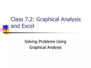
Class 7.2: Graphical Analysis and Excel Solving Problems Using Graphical Analysis
Learning Objectives • Learn to use tables and graphs as problem solving tools • Learn and apply different types of graphs and scales • Prepare graphs in Excel • Be able to edit graphs • Be able to plot data on log scale • Be able to determine the best-fit equations for linear, exponential and power functions
Exercise • Enter the following table in Excel • You can make your tables look nice by formatting text and borders
1 km Linear scale: Length (km) 1 km 10 km Log scale: Length (km) Axis Formats (Scales) • There are three common axis formats: • Rectilinear: Two linear axes • Semi-log: one log axis • Log-log: two log axes
Use of Logarithmic Scales • A logarithmic scale is normally used to plot numbers that span many orders of magnitude
Creating Log Scales in Excel • Exercise (2 min): Create a graph using x and y1 only.
Creating Log Scales in Excel • Now modify the graph so the data is plotted as semi-log y • This means that the y-axis is log scale and the x-axis is linear. • Right click on the axis to be modified and select “format axis”
Creating Log Scales in Excel • On the Scale tab, select logarithmic • “OK” • Next, go to Chart Options and select the Gridlines tab. Turn on (check) the Minor gridlines for the y-axis. • “OK”
Exercise (8 min) • Copy and Paste the graph twice. • Modify one of the new graphs to be semi-log x • Modify the other new graph to be log-log • Note how the scale affects the shape of the curve.
Result: log-log New Graph 10000 1000 y1 100 y1 10 1 1 10 100 1000 10000 x
Equations • The equation that represents a straight line on each type of scale is: • Linear (rectilinear): y = mx + b • Exponential (semi-log): y = bemx or y = b10mx • Power (log-log): y = bxm • The values of m and b can be determined if the coordinates of 2 points on THE BEST-FIT LINE are known: • Insert the values of x and y for each point in the equation (2 equations) • Solve for m and b (2 unknowns)
Equations (CAUTION) • The values of m and b can be determined if the coordinates of 2 points on THE BEST-FIT LINE are known. • You must select the points FROM THE LINE to compute m and b. In general, this will not be a data point from the data set. The exception - if the data point lies on the best-fit line.
Consider the data set: X Y 1 4 2 8 3 10 4 12 5 11 6 16 7 18 8 19 9 20 10 24
Team Exercise (3 minutes) • Using only the data from the table, determine the equation of the line that best fits the data. • When your team has completed this exercise, have one member write it on the board. • How well do the equations agree from each team? • Could you obtain a better “fit” if the data were graphed?
Which data points should be used to determine the equation of this best-fit line?
Which data points should be used to determine the equation of this best-fit line?
Comparing Results • How does this equation compare with those written on the board (i.e- computed without graphing) ? • CONCLUSION: NEVER try to fit a curve (line) to data without graphing or using a mathematical solution ( i.e – regression)
What about semi-log graphs? • Remember, straight lines on semi-log graphs are EXPONENTIAL functions.
What about log-log graphs? • Remember, straight lines on log-log graphs are POWER functions.
Example • Points (0.1, 2) and (6, 20) are taken from a straight line on a rectilinear graph. • Find the equation of the line, that is use these two points to solve for m and b. • Solution: 2 = m(0.1) + b a) 20 = m(6) + b b) Solving a) & b) simultaneously: m = 3.05, b = 1.69 Thus: y = 3.05x + 1.69
Pairs Exercise (10 min) • FRONT PAIR: • Points (0.1, 2) and (6, 20) are taken from a straight line on a log-log graph. • Find the equation of the line, ie - solve for m and b. • BACK PAIR: • Points (0.1, 2) and (6, 20) are taken from a straight line on a semi-log graph. • Find the equation(s) of the line, ie - solve for m and b.
Interpolation • Interpolation is the process of estimating a value for a point that lies on a curve between known data points • Linear interpolation assumes a straight line between the known data points • One Method: • Select the two points with known coordinates • Determine the equation of the line that passes through the two points • Insert the X value of the desired point in the equation and calculate the Y value
Individual Exercise (5 min) • Given the following set of points, find y2 using linear interpolation. (x1,y1) = (1,18) (x2,y2) = (2.4,y2) (x3,y3) = (4,35)
Assignment #13 • DUE: • TEAM ASSIGNMENT • See Handout