Estimating Impacts Using Revealed Preferences: Travel Cost Model

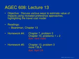
1. AGEC 608: Lecture 13 • Objective: Discuss various ways to estimate value of impacts using revealed preference approaches, highlighting the travel cost model • Readings: • Boardman, Chapter 13 • Homework #4: Chapter 7, problem 3 Chapter 10, problems 1 + 2due: next class • Homework #5: Chapter 13, problem 3 more T.B.A. due: April 24

2. Indirect estimation of demand • Main idea is to estimate “shadow prices” of goods based on observed behavior, when the market for the primary good does not exist. • Six main methods: • Market analogy method • Intermediate good method • Asset valuation method • Hedonic price method • Travel cost method • Defensive expenditure method

3. 1. Market analogy method Idea: use price or expenditure of an analogous good private good to value a public good Example: use price or expenditure on private housing as proxy for value of public housing Drawbacks: WTP > value of public good price of private good > WTP for public good

4. 2. Intermediate good method Approach: project produces intermediate good that is not sold in a market (e.g. job training) Impute the value provided to the “downstream” activity as: annual benefit = NI(with project) – NI (without) examples: wages with and without training agriculture with and without irrigation

5. 3. Asset valuation method Approach: look at differences in or changes in prices of assets associated with a project Example: value of good public schools = difference between price of housing in districts with and without good public schools (closely related to the hedonic pricing method)

6. 4. Hedonic price method Approach: value attribute or change in attribute when its value is capitalized into the price of an asset (often housing) Example: value of proximity to a school Step 1: regression P = b0SQFTb1CONTYPEb2DISTANCEb3ec Value of proximity R = b3P/DISTANCE Step 2: relate R to WTP R = W(DISTANCE, Y, Z), where Y = income, Z = hh charac.

7. Hedonic wage example Construction work is risky, and the riskiest jobs have wage premia. What if workers are willing to accept a 1/1000 annual risk of death to take a job that pays $1200 more per year? What is the value of one “statistical life”?

8. Calculating the hedonic wage Workers are willing to accept a 1/1000 annual risk of death to take a job that pays $1200 more per year. $1,200 * 1000 = $1,200,000 Therefore, 1000 people have a collective willingness to accept $1.2 million to be exposed to the death of one individual.

9. 5. Travel cost method Typically used for valuing recreation sites Approach: assume price “paid” to visit a sight includes time and cost of getting there. Use data on visitation to assign a total value to a sight. Drawbacks: econometric problems

10. 6. Defensive expenditure method Approach: use expenditure that occurs in response to something undesirable as the value of removing the undesirable feature Examples: value of reducing pollution = cost of cleaning windows value of clean water = cost of bottled water Drawbacks: defensive measures tend to underestimate benefits people tend to quickly adjust to undesirable changes

11. Travel cost model: example 1 5 locations 1 recreation site{A,B,C,D,E} B A D C E

12. Example 1: Visitation data Location Cost # visits A 0 50 B 25 45 C 50 40 D 125 25 E 250 0

13. Construct a demand curve • E 250 TravelCost • D P = 250 -5Q • C B • A • 0 0 50 Number of visits

14. 250 • E P = 250 -5Q • TravelCost D • C 0 • B • A 0 25 50 Number of visits Demand curve can be used to find: 1. consumer surplus (TB) 2. impact of increased fees

15. Example 2: Visitation data Location Cost # visits A 0 50 B 25 25 C 50 30 D 125 15 E 250 5

16. Example 2: Visitation data Regression model: dependent variable: visits independent variable: price visits = a + b*price visits = 38.25 – 0.147p (6.42) (3.15) N=5, R2=0.77

17. Construct a demand curve