Download
1 / 54
540 likes | 685 Vues
Relationship between mobility and diameter of singly charged spherical symmetric aerosol particles. Hannes.Tammet@ut.ee Workshop presentation 20120201. Introduction:. concept of diameter, mobility and mobility model, basic theoretical models, who made the Millikan model? ISO15900,

E N D
Relationship betweenmobility and diameterof singly chargedspherical symmetricaerosol particles Hannes.Tammet@ut.ee Workshop presentation 20120201
Introduction: • concept of diameter, • mobility and mobility model, • basic theoretical models, • who made the Millikan model? • ISO15900, • updating the Millikan model, • why the new modelsdo’nt have success? ? 2/54
from: Kulkarni, Baron Willeke Aerosol measurment A selection of diameters ..... .......volume diameter (Larriba et al. 2011, AST 45, 453-467) All these definitions expect that the diameter of a spherical particle is a well defined quantity. 3/54
Nanoparticles have “atmospheres”,no solid surface Density functions oftwo colliding nanoparticles 4/54
A similar problem: Atomic radii are required when assembling the crystal models. The radius of the same atom is a variable depending on the bonds. E.g. Na in the metallic natrium is much bigger than in a NaCl crystal. Slater (1964) proposed a specific mean radius as a universal parameter: Atom H O N Na Cs 2×RS:nm 0.05 0.12 0.13 0.36 0.52 The Slater radius of an orbital is the distance where the density of probability to find the electron has maximum. However the mean square deviation of real distances in crystals from the Slater distances is still about 0.012 nm. 5/54
Mass diameter NB: ρ = density of bulk matter ρ = density of particle matter An array of packed spheres has the density of 0.52 ρ in case of the simple cubic latticeand 0.74 ρin case of the closest packing. Mason, E.A. (1984) Ion mobility: its role in plasma chromatography.In Plasma Chromatography (Edited by T.W. Carr), 43–93.Plenum Press, New York and London. 6/54
Mobility and mobility model Precondition: the mean drift velocity v is proportional to the drag force F. Mechanical mobility B = v/F, electrical mobility Z = v/EF = Eqfollows inZ = qB. We haveq = eandZ = eB. A model of mobility is an algorithm that uses parameters of the particle and the air (pressure, temperature, diameter etc.) and issues an estimate of the particle mobility: Z ≈ ZM = fM (p, T, d) or Z ≈ ZM = fM (p, T,…, d). The inverse model d ≈ dM = gM(p, T, Z) is to be mathematically derived from the direct algorithm. 7/54
Epstein (1924) calculated effect of diffuse impacts on drag of about s = 1.32 s Theoretical basic models The Newton model of drag is nonlinear crosssection dynamicpressure Speed and fictive mechanical mobility F v Stokes model of drag is linear Rigid sphere model by Chapman ja Enskogin first approximation Ω = Ω(1,1) and Ω(1,1) = πr2 8/54
Mobility diameter Mobility diameter is defined as the diameter of a hard sphere of the same mobility as the considered particle. Thus the mobility diameter of a spherical particle is just the same as its geometric diameter. Sometimes the mobility diameter is considered asa value dM issued by a specific mobility model dM = gM (p, T, Z), where gM is inverse function of the model M and Z is measured mobility. The choice of the specific model is free, one could choose even plain Stokes or Newton. Thus dM should not be considered as a physical quantity. It is a specific estimate of the diameter. 9/54
Wang, H. (2009) Transport properties of small spherical particles. Ann. N.Y. Acad. Sci. 1161, 484–493. 10/54
Comparison of models B : (m/s) / fN is the speed (m/s) caused by force of 10-15 N Z : cm2 / (V s) = 1.6022 × B : (m/s) / fN Values of parameters (gaas = õhk, mõõtühikud SI): p = 101325 Pa, T = 273.15 K, ρp = 2000 , ρg = 1.293, k = 1.38E-23, η = 1.736E-5 dg = 3.74E-10, ng = 2.687E+25, mg = 4.809E-26, 11/54
??? There is no likelihood man can ever tap the power of the atom. The glib supposition of utilizing atomic energy when our coal has run outis acompletely unscientific Utopian dream, a childish bug-a-boo. Nature has introduced a few fool-proof devices into the great majority of elements that constitute the bulk of the world, and they have no energy to give up in the process of disintegration. 13/54
Who made the Millikan model? Robert Andrews Millikan MoritzWeber Ebenezer Cunningham Martin Knudsen (no Jens) 16/54
Millikan model Millikan 1923: A = 0.864 B = 0.29 C = 1.25 Davies 1945: A = 1.257 B = 0.400 C = 0.55 Allen & Raabe 1985: A = 1.142 B = 0.558 C = 0.999 Tammet 1995: A = 1.2 B = 0.5 C = 1 Kim et al. 2005: A = 1.165 B = 0.483 C = 0.997 Jung et al. 2011: A = 1.165 B = 0.480 C = 1.001 Kim, J.H., Mulholland, G.W, Kukuck, S.R., Pui, D.Y.H. (2005)Slip correction measurements of certified PSL nanoparticles using a nanometer differential mobility analyzer (Nano-DMA) for Knudsen number from 0.5 to 83.J. Res. Natl. Inst. Stand. Technol. 110, 31–54. 17/54
Knudsen Martin Hans Christian Knudsen (1871 - 1949) was a Danish physicist at the Technical University of Denmark. He is primarily known for his study of molecular gas flow and the development of the Knudsen cell, which is a primary component of molecular beam epitaxy systems. His book, The Kinetic Theory of Gases (London, 1934), contains the main results of his research. From basic physics: what is the measure of the vacuum? l – free path x – flight range NB: nanometer particles in atmospheric air are surrounded with vacuum. x 18/54
(Pseudo)problem of free path See Jennings (1988) In old books l = 3D / v ≈ 90 nm, in new books l ≈ 2D / v≈ 60 nm Now the free path is everywhere in combination with one of the coefficients A, B, C and effect of changed value of l can be exactly compensated with a change in values of A, B, C. Jung et al. 2011: A = 1.165 B = 0.480 C = 1.001Updated Millikan: A = 1.296 B = 0.435 C = 0.833Millikan 1923: A = 0.864 B = 0.29 C = 1.25 19/54
ISO15900 Sutherland, 1893 20/54
Updating the Millikan model Original model Z = ZMillikan (p, T, d) does not consider: ► polarization interaction between ions and gas molecules, ► size and mass of gas molecules, ► transition from diffuse scattering of molecules to the elastic-specular collisions. First update: the diameter complement Z = ZMillikan (p, T, d + Δd) Standard collision diameter of “air molecules” = 0.37 nm Tammet (1995) (at d → infinity):Δd →0.6 nm Fernandez de la Mora et al. (2003) : Δd = 0.53 nm Ku et al. (2009) :Δd = 0.3 nm Larriba et al. (2011) :Δd = 0.3 nm 21/54
Second update: Z = ZMillikan * Mass coefficient Mass coefficient = 23/54
A selection of newer models Tammet, H. (1995) Size and mobility of nanometer particles,clusters and ions. J. Aerosol Sci. 26, 459–475. Li, Z., Wang, H. (2003) Drag force, diffusion coefficient, and electric mobility of small particles. II. Application. Phys. Rev. E 68, 061207. Shandakov, S.D., Nasibulin, A.G., Kauppinen, E.I. (2005) Phenomenological description of mobility of nm- and sub-nm-sized charged aerosol particles in electric field. J. Aerosol Sci. 36, 1125–1143 . Wang, H. (2009) Transport properties of small spherical particles. Ann. N.Y. Acad. Sci. 1161, 484–493. 24/54
Bibliometry Citations in 2010 ja 2011 recorded in WebOfScience(paper by Ku et al. was published 2009) : Li and Wang (2003) 8 Ku et al. (2009)20 Tammet (1995) 26 Google search : all years 2007-2011 “Millikan diameter”43 14 “Tammetdiameter”32 6 25/54
Poor success of new models The model by Li and Wang (2003) is based on the most developed theory. However, Google did not find any application of this model in aerosol measurements. The same can be told about the model by Shandakov el al. (2005). Few references are found only inside of block references in introductions of the papers. Reasons? 1. No simple computing algorithm available. 2. No comprehensible interpretation available. 26/54
Poor success of new models The model by Tammet (1995) have had few applications. The detailed algorithm is available, but long and cumbersome. There is no simple interpretation. Mäkelä et al. (1996) made an attempt to find a simplified formal approximation: 27/54
End of the introduction Proposal and discussion of a new model
New approach In sake of convenience and accustomed interpretation:the new model is made up of the Millikan equation with a diameter complement. With an aim to take into account the peculiarities of d < 3 nm particles:the diameter complement is considered as a function of the particle mass diameter,and when required, of the air temperature and pressure: Δd = f (d) or Δd = f (p, T, d). (so far Δdwas considered as a constant) Problem: how to determine this function and how to assure simplicity of applications? 29/54
Determining of Δd = f (d) At the first glance it seems to be a similarity with the Cunningham-Knudsen-Weber-Millikan task to find a good approximation for the slip factor. However, there is a fundamental difference: ►slip factor depends on the Kn that can obtain high value in case of relatively large particles at low pressure, ►Δd depends immediately on the particle size and cannot be controlled by pressure. Thus the low pressure experiments with large particles are not helpful and the experiments should be made with sub-3 nm sperical particles of exactly known size. 0/54
Determining of Δd = f (d) 1. Get a reference table of precise measurements or an exact reference model of Z = f(d). The reference model may have no requirements for simple interpretation and computation. 2. Choose parameters of air p, T and a diameter d1, 3. Get the accurate mobility Z = Z (d1) from the reference table or compute it by means of the reference model. 4. Calculate by means of plain ISO15900 Millikan model (Δd = 0) a diameter d2 that corresponds to Z obtained in p.3. 5. Calculate the diameter complement Δd = d2 – d1 . Now the result of plain Millikan equation at d1 + Δd is exactly the same as the reference mobility. We will get different value of Δd for every d in the range of d < 3 nm and should compile a representative table of function Δd = f (d). 31/54
Determining of Δd = f (d) Next task is: to find a good approximation for the tabulated function Δd = f (d). The task is a bit similar to the Cunningham-Millikan problem of looking for approximation the slip correction factor. Unfortunately, we have no physical idea and the search for the approximation is considered as a formal procedure based on intuition and numerical methods of computational mathematics. A remark: The reference table of measurements of the function Δd = f (d) is strongly preferred. Such a table was not available when compiling the presentation and following examples are designed using a reference model. 32/54
The reference model The reference model was based on the Z = f(d) model by Tammet (1995) because the lack of well prepared alternatives. The original model was modified becausethe approximations of the air viscosity, free path and slip factor coefficients A, B, C should be the same in the Millikan equation and in the reference model. These approximations are prescribed in ISO15900. Exception:Standard values B = 0.483, C = 0.997 may be replaced with recent results B = 0.480, C = 1.001. These changes were entered into the algorithm and the result Tammet95m was used as a tentative reference model. 33/54
The reference model Z = f (p, T, ρ, q, d) function electrical_mobility_air {Tammet95m} (Millibar, Celsius, ParticleDensity {g cm-3, for cluster ions typically 2.08}, ParticleCharge {e, for cluster ions 1}, MassDiameter {nm} : real) : real; function Omega11 (x : real) : real; {*(1,1)*(T*) for (*-4) potential} var p, q : real; {and elastic-specular collisions} begin if x > 1 then Omega11 := 1 + 0.106 / x + 0.263 / exp ((4/3) * ln (x)) else begin p := sqrt (x); q := sqrt (p); Omega11 := 1.4691 / p - 0.341 / q + 0.181 * x * q + 0.059 end; end; const GasMass = 28.96; {amu} Polarizability = 0.00171; {nm3} a = 1.165; b = 0.48; c = 1.001; {the slip factor coefficients} ExtraDistance = 0.115 {nm}; TransitionDiameter = 2.48 {nm}; var Temperature, GasDiameter, Viscosity, FreePath, DipolEffect, DeltaTemperature, CheckMark, ParticleMass, CollisionDistance, Kn, Omega, s, x, y, r1, r2 : real; 34/54
The reference model begin if MassDiameter < 0.2 then {emergency exit} begin electrical_mobility_air := 1e99; exit; end; Temperature := Celsius + 273.15; r1 := Temperature / 296.15; r2 := 406.55 / (Temperature + 110.4); Viscosity {microPa s} := 18.3245 * r1 * sqrt (r1) * r2; FreePath {nm} := 67.3 * sqr (r1) * (1013 / millibar) * r2; ParticleMass {amu} := 315.3 * ParticleDensity * exp (3 * ln (MassDiameter)); DeltaTemperature := Temperature; repeat CheckMark := DeltaTemperature; GasDiameter {nm} := 0.3036 * (1 + exp (0.8 * ln (44 / DeltaTemperature))); CollisionDistance {nm} := MassDiameter / 2 + ExtraDistance + GasDiameter / 2; DipolEffect := 8355 * sqr (ParticleCharge) * Polarizability / sqr (sqr (CollisionDistance)); DeltaTemperature := Temperature + DipolEffect; until abs (CheckMark - DeltaTemperature) < 0.01; if ParticleCharge = 0 then Omega := 1 else Omega := Omega11 (Temperature / DipolEffect); Kn := FreePath / CollisionDistance; if Kn < 0.03 {underflow safe} then y := 0 else y := exp (- c / Kn); x := (273.15 / DeltaTemperature) * exp (3 * ln (TransitionDiameter / MassDiameter)); if x > 30 {overflow safe} then s := 1 else if x > 0.001 then s := 1 + exp (x) * sqr (x / (exp (x) - 1)) * (2.25 / (a + b) - 1) else {underflow safe} s := 1 + (2.25 / (a + b) - 1); electrical_mobility_air := 1.6022 * ((2.25 / (a + b)) / (Omega + s - 1)) * sqrt (1 + GasMass / ParticleMass) * (1 + Kn * (a + b * y)) / (6 * PI * Viscosity * CollisionDistance); end; 35/54
Experiment 1: Z = f (d)(p = 1013 mb) Millikan+ is the Millikan model for d + 0.3 nm as recommended byKu et al. (2009) Δd Studies of small ions and gas discharge estimate the mobilities of small molecular ions (d ≈ 0.4 nm) at standard conditions about 2.2 … 2.5 cm2V-1s-1 and less. Millikan+ issues about 4 cm2V-1s-1. 36/54
Experiment 3: Fitting of Δd = f (d) Z1 = fMillikanZ (p, T, d +fΔ1 (d)) Δd≈ fΔ1 (d) =k1 – k2 × exp (–k3 × (d – k4)2) – k5 / d EZ = (Z1 – Z0) / Z0 T = +10°C k1= 0.6 k2 = 0.22 k3 = 1.8 k4 = 1.2 k5 = 0.033 Five parameters, five zeros. 38/54
Experiment 3: Fitting of Δd = f (d) Z1 = fMillikanZ (p, T, d +fΔ1 (d)) Δd≈ fΔ1 (d) = 0.6 – 0.22 × exp (–1.8 × (d – 1.2)2) – 0.033 / d EZ = (Z1 – Z0) / Z0 39/54
Experiment 4: Temperature correction Z2 = fMillikanZ (p, T, d +fΔ2 (d, T)) fΔ2 (d, T) = 0.6 – 0.22 × exp (–1.8 × (d+ 0.001×T:C – 1.2)2) – 0.033 / d 40/54
Accuracy of approximation d = f (Z) Diameter is calculated by numerical inversion of the Millikan function. The error of approximation = deviation of the diameter calculated according to the approximate model from the diameter calculated according to the reference model. Estimating the error of approximation: • choose a value of d0, • calculate Z =freference (p, T, d0), • solve Z =fMillikanZ (p, T, d2 + fΔ2 (d2, T)) for d2. • absolute error = d2 – d0, • relative error = (d2 – d0) / d0. 41/54
Experiment 5:absolute error of approximation d = f (Z) 42/54
Experiment 7: pressure error of d = f (Z) ΔEZ = EZp – EZ1000 mb % 44/54
The end of the discussion Appendixes
Comparison of models Program A_tools, see http://ael.physic.ut.ee/tammet/A_tools/ Electrical mobility (cm2V-1s-1) at 1013 mb and 10 C: d:nm Millikan+ Tammet95 Reference Approx T95/Ref Mkn+/Ref Appr/Ref 0.6 2.48522 1.88764 1.92191 1.90759 0.9822 1.2931 0.9925 0.8 1.66449 1.38013 1.40518 1.41913 0.9822 1.1845 1.0099 1.0 1.19233 1.05643 1.07559 1.08827 0.9822 1.1085 1.0118 1.5 0.62271 0.55834 0.56846 0.56319 0.9822 1.0954 0.9907 2.0 0.38187 0.31324 0.31891 0.31930 0.9822 1.1974 1.0012 3.0 0.18597 0.15451 0.15730 0.15739 0.9823 1.1823 1.0006 5.0 0.07246 0.06379 0.06494 0.06511 0.9823 1.1159 1.0026 7.0 0.03839 0.03481 0.03543 0.03549 0.9824 1.0835 1.0017 10.0 0.01943 0.01804 0.01836 0.01838 0.9825 1.0587 1.0010 20.0 0.00514 0.00491 0.00499 0.00499 0.9830 1.0291 1.0003 50.0 0.00091 0.00088 0.00090 0.00090 0.9843 1.0112 1.0001 T95 is Tammet (1995) without corrections.Mkn+ is updated Millikan for d + 0.3 nm. 46/54
Pascal function Z_approx_air (millibar, Celsius, d {nm} : real) : real; {cm2 V-1 s-1, mathematical approximation of mobility Tammet95m} const a = 1.165; b = 0.48; c = 1.001; {Jung et al., 2011} var Viscosity, FreePath, Kn, r1, r2, y, dd : real; begin y := d + 0.001 * Celsius - 1.2; dd := d + 0.6 - 0.22 * exp (-1.8 * y * y) - 0.033 / d; r1 := (Celsius + 273.15) / 296.15; r2 := 406.55 / (Celsius + 383.55); Viscosity {microPa s} := 18.3245 * r1 * sqrt (r1) * r2; FreePath {nm} := 67.3 * sqr (r1) * (1013 / millibar) * r2; Kn := 2 * FreePath / dd; if Kn < 0.03 {underflow safe} then y := 0 else y := exp (- c / Kn); Z_approx_air := 1.6022 * (1 + Kn * (a + b * y)) / (3 * PI * Viscosity * dd); end; 47/54
Excel Sub Z_approx_air() ' HT 20120118 n = ActiveCell.Value For i = 0 To n - 1 mb = ActiveCell.Offset(i, -3).Value Celsius = ActiveCell.Offset(i, -2).Value d = ActiveCell.Offset(i, -1).Value y = d + 0.001 * Celsius - 1.2 dd = d + 0.6 - 0.22 * Exp(-1.8 * y * y) - 0.033 / d r1 = (Celsius + 273.15) / 296.15 r2 = 406.55 / (Celsius + 383.55) vi = 18.3245 * r1 * Sqr(r1) * r2 fp = 67.3 * r1 * r1 * (1013 / mb) * r2 Kn = 2 * fp / dd y = 0 If Kn > 0.03 Then y = Exp(-1.001 / Kn) Z = 1.6022 * (1 + Kn * (1.165 + 0.48 * y)) / (3 * 3.14159 * vi * dd) ActiveCell.Offset(i, 0) = Z Next i End Sub 48/54
Excel, inverse function Sub d_approx_air() ' HT 20120118 n = ActiveCell.Value For i = 0 To n - 1 mb = ActiveCell.Offset(i, -3).Value Celsius = ActiveCell.Offset(i, -2).Value Z = ActiveCell.Offset(i, -1).Value r1 = (Celsius + 273.15) / 296.15 r2 = 406.55 / (Celsius + 383.55) vi = 18.3245 * r1 * Sqr(r1) * r2 fp = 67.3 * r1 * r1 * (1013 / mb) * r2 c = 100 m = 0 OK = False While Not OK m = m + 1 d = (0.6 + Sqr(0.36 + 200 * c * Z)) / (c * Z) - 0.4 y = d + 0.001 * Celsius - 1.2 dd = d + 0.6 - 0.22 * Exp(-1.8 * y * y) - 0.033 / d Kn = 2 * fp / dd y = 0 If Kn > 0.03 Then y = Exp(-1.001 / Kn) test = 1.6022 * (1 + Kn * (1.165 + 0.48 * y)) / (3 * 3.14159 * vi * dd) c = (1.2 / (d + 0.4) + 200 / ((d + 0.4) * (d + 0.4))) / test OK = (Abs(test / Z - 1) < 0.000001) Or (m = 99) Wend If m > 99 Then d = 0 ActiveCell.Offset(i, 0) = d Next i End Sub 49/54
Excel, how to use? • Text of both macros is available in the document http://ael.physic.ut.ee/tammet/A_tools/Size-mobility-approx.pdf.Select and copy the text of one or two macros to the clipboard. • Open an Excel worksheet. Choose tools → macro → record new macro →store macro in this workbook → OK. A tiny recorder toolbar will appear.Remember the macro name and press the lower left button. The toolbar disappears and a new empty macro is saved. • Choose tools → macro → macros→name of the new empty macro→edit. VBA window will appear. Select full text of the empty macro and paste the text from the clipboard as a replacement. • Go back to the Excel worksheet, fill three neighbor columns in the worksheet with values of air pressure (mb), temperature (Celsius), and mobility (cm2V-1s-1), write number of rows to be processed into the cell just right of the first value of the mobility (see the example) and click this cell. NB: all data must be presented as values. • Choose tools → macro → macros→name of macro→RUN. 50/54