Download
1 / 23
230 likes | 248 Vues
Microphysics and boundary-layer research from long-term Doppler lidar observations. Robin Hogan Chris Westbrook, Tyrone Dunbar, Alan Grant, Ewan O’Connor, Anthony Illingworth, Stephen Belcher, Janet Barlow Dept of Meteorology, University of Reading. Resolving small-crystal controversy.

E N D
Microphysics and boundary-layer research from long-term Doppler lidar observations Robin Hogan Chris Westbrook, Tyrone Dunbar, Alan Grant, Ewan O’Connor, Anthony Illingworth, Stephen Belcher, Janet Barlow Dept of Meteorology, University of Reading
Resolving small-crystal controversy • Aircraft probe measurements: enormous numbers (1 cm-3) of tiny crystals < 50mm in cirrus • Cloud physics community is divided: are these real or an artefact due to break-up of larger particles on inlet? • Mitchell (2008) showed that if included in climate model, cloud albedo doubled real or fake? concentration size 50m Example time series: cirrus layer, falling at 0.5m/s BL aerosol
1.5-years of Doppler lidar data 1.5 years of data • Much better agreement when small crystals are not included • Suggests that they are not ubiquitous and are at least partially explained by shattering on aircraft probles • Westbrook & Illingworth (Geophys. Res. Lett., 2009) observations predicted range with small crystals predicted range without small crystals
Sometimes small-crystals do exist • Deep ice cloud • Single mode at cloud top • Nucleation at mid-levels • Bimodal when warmer than -15C • Large aggregates ~1 m/s • Small pristine plates ~0.3 m/s • Black crosses show Doppler lidar • Sometimes small ice can be seen to be falling from supercooled liquid layers • Westbrook et al. (2010, QJRMS) Doppler velocity m/s Chilbolton 35-GHz Copernicus radar
Two-color rain/drizzle sizing • Refractive index of water at 1.5 mm: 1.32 – 0.000135i • Half of energy absorbed over path of 600 mm • Refractive index of water at 905 nm: 1.33 – 0.000000561i • 1% of energy absorbed over path of 600 mm • Color ratio in rain and drizzle is monotonically related to size • Can derive rain rate and any other moment of the distribution • In particular, can predict the radar reflectivity for verification • In principle, could use the Doppler capability to also infer vertical wind • Similar to O’Connor et al. (JTECH 2005) for radar/lidar drizzle sizing • Sizing also possible in ice, although interpretation of the size measurement depends on particle habit • Westbrook et al. (2010, Atmos. Meas. Technol.)
Boundary layer dynamics Input of sensible heat “grows” a new cumulus-capped boundary layer during the day (small amount of stratocumulus in early morning) Convection is “switched off” when sensible heat flux goes negative at 1800 • Hogan et al. (QJRMS 2009) Surface heating leads to convectively generated turbulence
Comparing variance to previous studies • Lidar temporal resolution of ~30 s • Smallest eddies not detected, so add them using -5/3 law • Only valid in convective boundary layers where part of the inertial subrange is detected • Normalize variance by convective velocity scale • Reasonable agreement with Sorbjan (1980) and Lenschow et al. (1989) New contribution to variance
Skewness • Skewness defined as • Positive in convective daytime boundary layers • Agrees with aircraft observations of LeMone (1990) when plotted versus the fraction of distance into the boundary layer • Useful for diagnosing source of turbulence
11 April 2007 Longwave cooling Positively buoyant plumes generated at surface: normal convection and positive skewness Cloud Negatively buoyant plumes generated at cloud top: upside-down convection and negative skewness Height Height Shortwave heating Potential temperature Potential temperature Stratocumulus cloud
Inferring sensible heat flux • Vertical wind variance matches what would be predicted from measured surface sensible heat flux H (via w*) • Over urban areas it is impossible to measure a representative H using eddy correlation • Tyrone Dunbar, Stephen Belcher and Janet Barlow are developing a technique to infer H from variance of vertical wind Optimal estimation technique to find H and h that best fit sw2(z) Reasonable fit to sonic over Chilbolton
Estimating TKE dissipation rate • Can estimate e from variance in vertical velocity over ~1 min, and horizontal wind-speed • O’Connor et al. (2010, submitted to JTECH) • Backscatter • Dissipation rate • Error in dissipation rate - In-situ validation from tethered balloon
Lots of uses for 1.5-mm Doppler lidar • Properties of small crystals • Microphysics of mixed-phase clouds • Size of raindrops and large ice particles (with two lidars) • Vertical wind at liquid cloud base for activation of CCN • TKE dissipation rate – evaluation of large-eddy models • Inferring sensible heat flux over urban areas • Determining source of turbulence (top-down or bottom-up) • Evaluating boundary layer parameterizations in GCMs/NWP • Evaluating vertical velocity representation in dispersion models
Skewness in convective BLs • Both model simulations and laboratory visualisation show convective boundary layers heated from below to have narrow, intense updrafts and weak, broad downdrafts, i.e. positive skewness Narrow fast updrafts Wide slow downdrafts Courtesy Peter Sullivan NCAR
Why is skewness positive? • Consider TKE budget: • Vertical flux of TKE is • So skewness positive when TKE transported upwards by turbulence Stull TKE destroyed by dissipation & buoyancy suppression at BL top TKE transported upwards by turbulence TKE generated by shear and buoyancy in lower BL Transport
...a alternative related explanation • Updraft regions of large eddies have more intense small-scale turbulence than the downdraft regions • This leads to an asymmetric velocity distribution • Will test this later... Large eddies only All eddies
Cospectrum Vertical wind from 11 April 2007 at time of transition • The cospectrum, Cww2: • Defined as the complex conjugate of FFT of w’ multiplied by FFT of w’ 2 • Can be thought of as a spectral decomposition of the third moment: • Hunt et al. (1988) showed that it goes as freq-2 in intertial subrange Skewness dominated by larger (20 minute timescale) eddies
Closed-cell stratocu. • Previous studies have shown updraft/downdraft asymmetry in stratocumulus at the largest scales • Puzzle as to why aspect ratio of cells is as much as 30:1 Shao & Randall (JAS 1996)
Aircraft vs LES LES: Moeng and Wyngaard (1988) Aircraft observations: LeMone (1990)
Upside-down Carson’s model • If all the physics is the same but inverted, we can apply Carson’s model to predict the growth of the cloud-top-cooling driven mixed layer • With longwave cooling rate of H = 30 W m-2 and lapse rate of g = 1 K km-1, we estimate growth of 1.1 km in 3 hours, approximately the same as observed
Comparison of top-down and bottom-up • Variance of vertical wind • Good agreement with previous studies if H = 30 W m-2 • Variance peaks in upper third of BL: agrees with Lenschow et al.’s fit provided theirs is inverted in height • Skewness • Very good agreement with the fit of LeMone (1990) to aircraft data provided hers is inverted in sign and height • Hogan et al. (QJRMS 2009)